Automatic Differentiation: Forward and Reverse
Update 1 (2022/05/11): See Hacker News discussion here.
Update 2 (2022/07/17): Fixed a typo in evaluation traces pointed out by Walter Ehren. Thanks!
Update 3 (2023/02/09): Fixed a typo in tables pointed out by John Snyder. Thanks!
Deriving derivatives is not fun. In this post, I will deep dive into the methods for automatic differentiation (abbreviated as AD by many). After reading this post, you should feel confident with using the various AD techniques, and hopefully never manually calculate derivatives again. Note that this post is not a comparison between AD libraries. For that, a good starting point is here.
Why Automatic Differentiation?
Automatic differentiation (AD) is a natural continuation of scientists and engineers’ pursuit for mechanizing computation. After all, we learn how to take derivatives by memorizing a set of rules. Why can’t computers do the same thing?
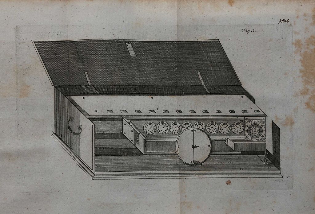
Figure 1: Leibniz’s drawing of his calculating machine, appeared in Miscellanea Berolensia ad incrementum scientiarum (1710) (source). This machine was supposed to be able to conduct addition, subtraction, multiplication and division. Unfortunately the prototype never worked properly.
Nevertheless, if you just simply follow the rules and symbolically solve for derivatives, the results you get will be deep in the expression hell. Consider the product rule we are all familiar with:
\begin{align} \frac{d}{d x}(f(x) g(x)) = \left(\frac{d}{d x} f(x)\right) g(x)+f(x)\left(\frac{d}{d x} g(x)\right) \end{align}
Assume that we are not conducting any simplification along the way.
By simply following the product rule, we are multiplying the number of common terms in both \(f(x)\) and \(\frac{d}{dx}f(x)\), and \(g(x)\) and \(\frac{d}{dx}g(x)\) by two.
Essentially, this well result in a tree-like structure where the number of terms increase exponentially.
Table 1 shows the results of applying symbolic differentiation using MATLAB’s diff(f,x) function without simplification.
Notice how the number of terms drastically increase, and how there are a repetition of the same terms in the derivatives’ expressions (which will come in handy when we discuss the algorithms for AD).
| \(f(x)\) | \(\frac{d}{dx} f(x)\) from MATLAB R2021a’s diff(f, x) |
|---|---|
| 4(x-1)(x-2) | 8x-12 |
| 4(x-1)(x-2)(x-3) | 4(x - 2)(x - 3) + (4x - 4)(x - 2) + (4x - 4)(x - 3) |
| 4(x-1)(x-2)(x-3)(x-4) | (4x - 4)(x - 2)(x - 3) + (4x - 4)(x - 2)(x - 4) + (4x - 4)(x - 3)(x - 4) + 4(x - 2)(x - 3)(x - 4) |
So what if we find derivatives numerically? After all, in most applications we don’t care about the forms of the derivatives, only the final values. Perhaps we can try the finite difference method. It is essentially the numerical approximation to the definition of gradients. Given a scalar multivariate function \(f: \mathbb{R}^{n} \rightarrow \mathbb{R}\), we can approximate the gradients as
\begin{align} \frac{\partial f(\mathbf{x})}{\partial x_{i}} \approx \frac{f\left(\mathbf{x}+h \mathbf{e}_{i}\right)-f(\mathbf{x})}{h} \end{align}where \(\mathbf{e}_{i}\) are the i-th unit vector and \(h\) is a small number. This is the so-called forward difference method.
![]()
Figure 2: Errors of forward difference method at different \(h\). At small \(h\), round off errors dominate, and at large \(h\), truncation errors dominate.
There are a few issues with this method. First, it requires \(O(n)\) work for n-dimensional gradients, which is prohibitive for neural networks with millions of learnable parameters. It is also plagued by numerical errors. Specifically, round-off errors (errors caused by using finite-bit floating point representations) and truncation errors (the difference between the analytical gradients and the numerical gradients). At small \(h\), round-off errors dominate. At large \(h\), truncation errors dominate (see Fig. 2). Such errors might be significant in ill-conditioned problems, causing numerical instabilities.
Automatic differentiation, on the other hand, is a solution to the problem of calculating derivatives without the downfalls of symbolic differentiation and finite differences. The key idea behind AD is to decompose calculations into elementary steps that form an evaluation trace, and combine each step’s derivative together through the chain rule. Because of the use of evaluation traces, AD can differentiate through not only closed-form calculations, but also control flow statements used in programs. Regardless of the actual path taken, at the end numerical computations will form an evaluation trace which can be used for AD.
In the rest of this post, I introduce the definition of evaluation traces, and the two modes of AD: forward and reverse. I accompany the discussion with a implementation written in Rust.
Evaluation Traces
To decompose the functions into elementary steps, we need to construct their evaluation traces. You can view these traces as a recording of the steps you take to reach the final results. Let’s take a look at an example function \(f: \mathbb{R}^{n} \rightarrow \mathbb{R}^{m}\) where \(n=2\) and \(m=1\) taken from Griewank and Walther 1:
\begin{align} y=\left[\sin \left(x_{1} / x_{2}\right)+x_{1} / x_{2}-\exp \left(x_{2}\right)\right] \left[x_{1} / x_{2}-\exp \left(x_{2}\right)\right] \end{align}Define the following variables:
- \(v_{i-n} = x_{i}\), \(i=1, \ldots, n\) are the input variables,
- \(v_{i}\), \(i=1,\ldots,l\) are the intermediate variables,
- \(y_{m-i} = v_{l-i}\), \(i=m-1, \ldots, 0\) are the output variables.
Note that the numbering system used is arbitrary, as long as it is consistent.
Let’s now evaluate the function when \(x_{1} = 1.5\) and \(x_{2} = 0.5\), and record all the intermediate values.
| Intermediate Vars. | Expressions | Values |
|---|---|---|
| \(v_{-1}\) | \(x_1\) | \(1.5\) |
| \(v_{0}\) | \(x_2\) | \(0.5\) |
| \(v_{1}\) | \(v_{-1} / v_{0}\) | \(3.0000\) |
| \(v_{2}\) | \(\sin{(v_{1})}\) | \(0.1411\) |
| \(v_{3}\) | \(\exp(v_{0})\) | \(1.6487\) |
| \(v_{4}\) | \(v1 - v3\) | \(1.3513\) |
| \(v_{5}\) | \(v2+v4\) | \(1.4924\) |
| \(v_{6}\) | \(v5 \cdot v4\) | \(2.0167\) |
\(v_{6}\) is the final output variable \(y\), which equals to \(2.0167\). Some also call this evaluation trace the Wengert list, which is named after the author of the 1964 paper A Simple Automatic Derivative Evaluation Program. Note that there is nothing special about this list. In fact, you can probably represent it as a list in Python if you want.
Graphically, we can also represent it as a directed acyclic graph, where the variables are the nodes of the graph, and edges represent the algebraic relationships.
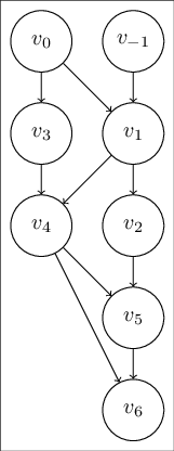
Figure 3: Computation Graph of Table 2, for \(y=\left[\sin \left(x_{1} / x_{2}\right)+x_{1} / x_{2}-\exp \left(x_{2}\right)\right] \left[x_{1} / x_{2}-\exp \left(x_{2}\right)\right]\)
Comparing to the table format, this graph shows the logical dependencies of each of the intermediate variables on the evaluation trace better. For example, if we want to compute \(v_{5}\), we have to have computed \(v_{4}\) and \(v_{2}\).
A logical next step for finding the defivatives of \(y\) with respect to \(x_{1}\) and \(x_{2}\) is to follow the evaluation trace, and simple calculate the derivatives one intermediate variable at a time. This leads us to the forward mode automatic differentiation algorithm.
Forward Mode
Accumulating the Tangent Trace
Let’s say we want to calculate the partial derivative of \(y\) with respect to \(x_{1}\), with \(x_{1} = 1.5\) and \(x_{2} = 0.5\). As we mentioned above, we can try do it one intermediate variable at a time. Note that we are only calculating the numerical value of the derivative. For each \(v_{i}\), we calculate \(\dot{v}_{i} = \frac{\partial v_{i}}{\partial x_{1}}\). Let’s try a few variables to see how it goes:
\begin{align} \dot{v}_{-1} &= \frac{\partial x_{1}}{\partial x_{1}} = 1.0 \\ \dot{v}_{0} &= \frac{\partial x_{2}}{\partial x_{1}} = 0 \\ \dot{v}_{1} &= \frac{\partial (v_{-1} / v_{0}) }{\partial x_{1}} = \dot{v}_{-1} (v_{0}^{-1}) + \dot{v}_{0} (-v_{-1} v_{0}^{-2}) = 1.00 / 0.50 = 2.00 \\ \dot{v}_{2} &= \frac{\partial (\sin{(v_{1})}) }{\partial x_{1}} = \cos(v_{1}) \dot{v_{1}} = -0.99 \times 2.00 = -1.98 \end{align}For these calculations, we are simply applying chain rules with basic derivatives. Note that how \(\dot{v}_{i}\) only depends on the derivatives and values of the earlier variables. We can now augment Table 2 to include the derivatives.
| Intermediate Vars. | Values | Derivatives |
|---|---|---|
| \(v_{-1}\) | \(1.5\) | \(1.0\) |
| \(v_{0}\) | \(0.5\) | \(0.0\) |
| \(v_{1}\) | \(3.0000\) | \(2.0\) |
| \(v_{2}\) | \(0.1411\) | \(-1.98\) |
| \(v_{3}\) | \(1.6487\) | \(0.0\) |
| \(v_{4}\) | \(1.3513\) | \(2.0\) |
| \(v_{5}\) | \(1.4924\) | \(0.02\) |
| \(v_{6}\) | \(2.0167\) | \(3.0118\) |
The values of the intermediate variables are sometimes called the primal trace, and the derivative values the tangent trace.
This generalizes nicely to a generic vector-valued function \(f: \mathbb{R}^{n} \rightarrow \mathbb{R}^{m}\). Assume we are trying to evaluate the function at \(\mathbf{x} = \mathbf{a}, \mathbf{a} \in \mathbb{R}^{n}\). In that case, the Jacobian matrix is in the form of
\begin{align} \mathbf{J}_{f}=\left.\left[\begin{array}{ccc} \frac{\partial y_{1}}{\partial x_{1}} & \cdots & \frac{\partial y_{1}}{\partial x_{n}} \\ \vdots & \ddots & \vdots \\ \frac{\partial y_{m}}{\partial x_{1}} & \cdots & \frac{\partial y_{m}}{\partial x_{n}} \end{array}\right]\right|_{\mathbf{x}=\mathbf{a}} \end{align}and each column consists of
\begin{align} \dot{y}_{j}=\left.\frac{\partial y_{j}}{\partial x_{i}}\right|_{\mathbf{x}=\mathbf{a}}, j=1, \ldots, m \end{align}which are the partial derivatives of \(y_{j}\) with respect to each \(x_{i}\). So we can obtain the columns one by one by setting the corresponding \(\dot{x}_{i} = 1\) and setting the other entries zero. This opens some interesting techniques. For example, if we want to compute the Jacobian-vector product with \(\mathbf{r}\), we can simply set \(\dot{\mathbf{x}}=\mathbf{r}\) instead of a unit vector:
\begin{align} \mathbf{J}_{f} \mathbf{r}=\left[\begin{array}{ccc} \frac{\partial y_{1}}{\partial x_{1}} & \cdots & \frac{\partial y_{1}}{\partial x_{n}} \\ \vdots & \ddots & \vdots \\ \frac{\partial y_{m}}{\partial x_{1}} & \cdots & \frac{\partial y_{m}}{\partial x_{n}} \end{array}\right]\left[\begin{array}{c} r_{1} \\ \vdots \\ r_{n} \end{array}\right]. \end{align}In terms of complexity, forward mode is on the order of \(O(n)\), where \(n\) is the dimension of the input vector. Hence, it will be a great choice for \(f: \mathbb{R} \rightarrow \mathbb{R}^{m}\), while performing poorly for \(f: \mathbb{R}^{n} \rightarrow \mathbb{R}\).
Using Dual Numbers
One popular way to implement forward mode AD is to use dual numbers. Dual numbers were introduced by William Clifford in 1873 through his paper Preliminary Sketch of Biquaternions. Clifford was studying how to extend Hamilton’s vectors to consider rotations around not only the origin, but any arbitrary lines in the 3-dimensional space. He called his extension on vectors rotors, and the sum of such rotors motors. He then introduces a symbol \(\omega\) to convert motors into vectors, and that \(\omega^{2} = 0\). His reasoning was purely geometric:
The symbol \(\omega\), applied to any motor, changes it into a vector parallel to its axis and proportional to the rotor part of it. … and if made to operate directly on a vector, reduces it to zero.
However, it turns out that dual numbers can be conveniently to represent differentiation.
Formally, we represent dual numbers as \(a + b\epsilon\). They follow the usual component-wise addition rule:
\begin{align} (a + b \epsilon) + (c + d \epsilon) = (a + c) + (b + d) \epsilon. \end{align}And their multiplications work like this (similar to complex numbers):
\begin{align} (a+b \epsilon)(c+d \epsilon)=a c+(a d+b c) \epsilon + db \epsilon^{2} = a c + (a d+b c) \epsilon, \end{align}with the rule that \(\epsilon^{2} = 0\).
The connection between dual numbers and differentiation becomes clear once we look at the Taylor series expansion. Given an arbitrary real function \(f : \mathbb{R} \rightarrow \mathbb{R}\), we can express its Taylor series expansion at \(x_{0}\) as
\begin{align} f(x)=f\left(x_{0}\right)+f^{\prime}\left(x_{0}\right)\left(x-x_{0}\right)+\cdots+\frac{f^{(n)}\left(x_{0}\right)}{n !}\left(x-x_{0}\right)^{n}+\mathcal{O}\left(\left(x-x_{0}\right)^{n+1}\right) \end{align}as long as the function is \(n+1\) times differentiable and has bounded \(n+1\) derivative. If we instead extend them to using dual numbers as inputs, it follows that
\begin{align} f(a + b \epsilon) =\sum_{n=0}^{\infty} \frac{f^{(n)}(a) b^{n} \epsilon^{n}}{n !}=f(a)+b f^{\prime}(a) \epsilon. \end{align}So if we set \(b=1\), we can get the derivative at \(x=a\) by taking the coefficient of \(\epsilon\) after evaluation:
\begin{align} \label{eq:dual-single-v} \tag{1} f(a + \epsilon) = f(a) + f^{\prime}(a) \epsilon \end{align}where we expanded the Taylor series at \(a\), and since \(\epsilon^{2} = 0\), all terms involving \(\epsilon^{2}\) and higher vanish. Under this formulation, addition works:
\begin{align} f(a + \epsilon) + g(a + \epsilon) &= f(a) + g(a) + (f^{\prime}(a) + g^{\prime}(a) ) \epsilon. \end{align}Multiplication works:
\begin{align} f(a + \epsilon) g(a + \epsilon) &= f(a) g(a) + (f^{\prime}(a) g(a) + f(a) g^{\prime}(a) ) \epsilon. \end{align}And chain rule works as expected:
\begin{align} f(g(a + \epsilon)) &=f(g(a) + g^{\prime}(a) \epsilon) \\ &=f(g(a)) + f^{\prime}(g(a)) g^{\prime}(a) \epsilon. \end{align}This essentially gives us the way to conduct forward mode AD: by using dual numbers, we can get the primal and tangent trace simultaneously.
So, how do we take this to higher dimensions? We simply add an \(\epsilon\) for each component. Assume a function \(f: \mathbb{R}^{n} \rightarrow \mathbb{R}\). We define a vector \(\boldsymbol{\epsilon} \in \mathbb{R}^{n}\) where \(\boldsymbol{\epsilon}_{i}^{2} = \boldsymbol{\epsilon}_{i} \boldsymbol{\epsilon}_{j} = 0\). If you write out the component-wise computation following Eq. \ref{eq:dual-single-v}, it follows that
\begin{align} \label{eq:dual-multi-v} \tag{2} f(\boldsymbol{a} + \boldsymbol{\epsilon}) = f(\boldsymbol{a}) + \nabla f(\boldsymbol{a}) \cdot \boldsymbol{\epsilon} \end{align}\(\nabla f(\boldsymbol{a}) \cdot \boldsymbol{\epsilon}\) can be interpreted as the directional derivative of \(f\) in the direction of \(\boldsymbol{\epsilon}\). Addition, multiplication and chain rule work as expected:
\begin{align} f(\boldsymbol{a} + \boldsymbol{\epsilon}) + g(\boldsymbol{a} + \boldsymbol{\epsilon}) &= f(\boldsymbol{a}) + g(\boldsymbol{a}) + (\nabla f(\boldsymbol{a}) + \nabla g(\boldsymbol{a}) ) \boldsymbol{\epsilon} \\ f(\boldsymbol{a} + \boldsymbol{\epsilon}) g(\boldsymbol{a} + \boldsymbol{\epsilon}) &= f(\boldsymbol{a}) g(\boldsymbol{a}) + (\nabla f(\boldsymbol{a}) g(\boldsymbol{a}) + f(\boldsymbol{a}) \nabla g(\boldsymbol{a}) ) \boldsymbol{\epsilon} \\ f(g(\boldsymbol{a} + \boldsymbol{\epsilon})) &=f(g(\boldsymbol{a})) + \nabla f(g(\boldsymbol{a})) \nabla g(\boldsymbol{a}) \boldsymbol{\epsilon} \end{align}For \(f : \mathbb{R}^{n} \rightarrow \mathbb{R}^{m}\), instead of using a vector of \(\epsilon\), we can use a matrix of \(\epsilon\). And for each row of that matrix, we follow the exact same rule as Eq. \ref{eq:dual-multi-v}.
Reverse Mode
Propagate From the End
Reverse mode automatic differentiation, also known as adjoint mode, calculates the derivative by going from the end of the evaluation trace to the beginning. The intuition comes from the chain rule. Consider a function \(y = f(x(t))\). From the chain rule, it follows that
\begin{align} \frac{\partial y}{\partial t} = \frac{\partial y}{\partial x} \cdot \frac{\partial x}{\partial t} \end{align}The two terms on the right-hand side can be seen as going backwards: \(\frac{\partial y}{\partial x}\) can be determined once we calculate \(y\) from \(x\), and \(\frac{\partial x}{\partial t}\) can be calculated once we calculate \(x\) from \(t\). Extending this to multivariate functions, we have the multivariate chain rule:
Theorem 1: Suppose \(g: \mathbf{R}^{n} \rightarrow \mathbf{R}^{m}\) is differentiable at \(a \in \mathbf{R}^{n}\) and \(f: \mathbf{R}^{m} \rightarrow \mathbf{R}^{p}\) is differentiable at \(g(a) \in \mathbf{R}^{m}\). Then \(f \circ g: \mathbf{R}^{n} \rightarrow \mathbf{R}^{p}\) is differentiable at \(a\), and its derivative at this point is given by \[ D_{a}(f \circ g)=D_{g(a)}(f) D_{a}(g). \]
The proof of it can be found in Appendix A4 of Vector Calculus, Linear Algebra, and Differential Forms: a Unified Approach by John H. Hubbard and Barbara Burke Hubbard. For example, for a function \(F(t) = f(g(t)) = f(x(t), y(t))\) where \(f : \mathbf{R}^{2} \rightarrow \mathbf{R}\) and \(g : \mathbf{R} \rightarrow \mathbf{R}^{2}\), we have
\begin{align} D_{a}(f \circ g)=D_{a}(F)=\frac{d F}{d t} \\ D_{g(a)}(f)=\left[\begin{array}{ll} \frac{\partial f}{\partial x} & \frac{\partial f}{\partial y} \end{array}\right] \\ D_{a}(g)=\left[\begin{array}{l} \partial x / \partial t \\ \partial y / \partial t \end{array}\right] \end{align}So it follows
\begin{align} \frac{d F}{d t} = \left[\begin{array}{ll} \frac{\partial f}{\partial x} & \frac{\partial f}{\partial y} \end{array}\right] \left[\begin{array}{l} \partial x / \partial t \\ \partial y / \partial t \end{array}\right] = \frac{\partial f}{\partial x} \frac{\partial x}{\partial t} + \frac{\partial f}{\partial y} \frac{\partial y}{\partial t} \end{align}Applying this idea to automatic differentiation, we have the reverse mode. To calculate derivatives in this mode, we need to conduct two passes. First, we need to do a forward pass, where we obtain the primal trace (Table 2). We then propagate the partials backward to obtain the desired derivatives (following the chain rule). Let’s go back to our example before to see reverse mode in action. Consider again the function
\begin{align} y=\left[\sin \left(x_{1} / x_{2}\right)+x_{1} / x_{2}-\exp \left(x_{2}\right)\right] \left[x_{1} / x_{2}-\exp \left(x_{2}\right)\right]. \end{align}Following the same way of assigning intermediate variables as in Table 2 and in Fig. 3, we can assemble an adjoint trace. An adjoint \(\bar{v}_{i}\) is defined as
\begin{align} \bar{v}_{i} = \frac{\partial y_{j}}{\partial v_{i}}, \end{align}which is equivalent to the product of all the partials from \(y_{j}\) up until \(v_{i}\). We start from the last variable \(v_{6} = y\):
\begin{align} \bar{v}_{6} &= \frac{\partial y}{\partial v_{6}} = 1 \\ \bar{v}_{5} &= \frac{\partial y}{\partial v_{5}} = \bar{v}_{6} \frac{\partial v_{6}}{\partial v_{5}} = 1 \times v_{4} = 1.3513 \\ \bar{v}_{4} &= \frac{\partial y}{\partial v_{4}} = \frac{\partial y}{\partial v_{5}} \frac{\partial v_{5}}{\partial v_{4}} + \frac{\partial y}{\partial v_{6}} \frac{\partial v_{6}}{\partial v_{4}} = \bar{v}_{5} \frac{\partial v_{5}}{\partial v_{4}} + \bar{v}_{6} \frac{\partial v_{6}}{\partial v_{4}} = 1.3513 + 1.4914 = 2.8437 \end{align}And repeat the same process for all the intermediate variables, we have Table 4 below.
| Intermediate Vars. | Values | Adjoints |
|---|---|---|
| \(v_{-1}\) | \(1.5\) | \(3.0118\) |
| \(v_{0}\) | \(0.5\) | \(-13.7239\) |
| \(v_{1}\) | \(3.0000\) | \(1.5059\) |
| \(v_{2}\) | \(0.1411\) | \(1.3513\) |
| \(v_{3}\) | \(1.6487\) | \(-2.8437\) |
| \(v_{4}\) | \(1.3513\) | \(2.8437\) |
| \(v_{5}\) | \(1.4924\) | \(1.3513\) |
| \(v_{6}\) | \(2.0167\) | \(1\) |
Note how we are able to obtain the adjoints of the input variables \(x\) and \(y\) (which are equivalent to the partial derivatives of \(f\) with respect to \(x\) and \(y\)) at the same time. For a function \(f : \mathbf{R}^{n} \rightarrow \mathbf{R}\), it takes only one application of reverse mode to compute the entire gradient. In general, if the dimension of the outputs is significantly smaller than that of inputs, reverse mode is a better choice.
diffomatic: My Implementation in Rust
It’s always fun to implement theories in actual code. In this section, I describe diffomatic, my attempt at implementing both forward and reverse mode automatic differentiation.
Note that in the current implementation, I only support first-order differentiation.
In addition, I have not spent any time optimizing the code. You can access the repo here.
During writing the code, I have referenced this repo and this blog post.
Forward Mode
To implement forward mode in Rust, I opt to create a structure to represent dual numbers:
pub struct DualScalar {
    pub v: f64,
    pub dv: f64,
}
The operations are then implemented on DualScalar,
following standard traits such as std::ops::{Add, Div, Mul, Neg, Sub}. For example,
impl Add for DualScalar {
    type Output = Self;

    fn add(self, rhs: Self) -> Self::Output {
        DualScalar {
            v: self.v + rhs.v,
            dv: self.dv + rhs.dv,
        }
    }
}
pub fn deriv(&self) -> f64 {
    self.dv.clone()
}
where the addition rule is implemented for the add(self, rhs: Self) function.
To access the derivative value, we have
And evaluating a function to get the derivative is done through the derivative<F>(func: F, x0: f64 ) function:
pub fn derivative<F>(func: F, x0: f64 ) -> f64
    where F : Fn(DualScalar) -> DualScalar,
{
    func(DualScalar{ v: x0, dv: 1.0}).deriv()
}
For multivariate functions, I simply represent the inputs as a Vec holding DualScalar.
pub fn gradient<F>(func: F, x0: &[f64]) -> Vec<f64>
    where F: Fn(&[DualScalar]) -> DualScalar,
{
    // To get all the partials, we set each var to have dv=1
    // and the others dv=0, and pass them through the function
    let mut inputs: Vec<DualScalar> = x0.iter().map(|&v| DualScalar { v: v, dv: 0. }).collect();
    (0..x0.len()).map(
        |i| {
            inputs[i].dv = 1.;
            let partial = func(&inputs).deriv();
            inputs[i].dv = 0.;
            partial
        }
    ).collect()
}
Note that we have to iterate through all the inputs by setting dv to be 1, then collect the partials.
For Jacobians, we obtain the columns one by one:
pub fn jacobian<F, const N: usize, const M: usize>(func: F, x0: &[f64]) -> SMatrix<f64, M, N>
    where F: Fn(&[DualScalar]) -> Vec<DualScalar>,
{
    // To get all the partials, we set each var to have dv=1
    // and the others dv=0, and pass them through the function
    let mut jacobian: SMatrix<f64, M, N> = SMatrix::zeros();
    let mut inputs: Vec<DualScalar> = x0.iter().map(|&v| DualScalar { v: v, dv: 0. }).collect();

    // every time we call the func we can get one column of partials
    for (i, mut col) in jacobian.column_iter_mut().enumerate() {
        inputs[i].dv = 1.;
        let col_result = func(&inputs);
        for j in 0..M {
            col[j] = col_result[j].dv;
        }
        inputs[i].dv = 0.;
    }

    return jacobian;
}
The API of these functions are pretty straightforward:
// API for forward mode
//
// derivative(f, x)
let f1_test = |x: fdiff::DualScalar| x * x;
let f1_result: f64 = fdiff::derivative(f1_test, 2.0);
println!("Derivative of f(x) = x^2 at {} is {}", 2.0, f1_result);

// gradient(f, x)
let f2_test = |x: &[fdiff::DualScalar]| x[0] + x[1];
let f2_result: Vec<f64> = fdiff::gradient(f2_test, vec![1., 2.].as_slice());
println!("Gradient of f(x,y) = x + y at ({}, {}) is {:?}", 1.0, 2.0, f2_result);

// jacobian(f, x)
// f(1) = x^2 * y
// f(2) = x + y
let f3_test = |x: &[fdiff::DualScalar]| {
    vec![x[0] * x[0] * x[1], x[0] + x[1]]
};
let f3_result: SMatrix<f64, 2, 2> = fdiff::jacobian(f3_test, vec![1., 2.].as_slice());
println!("Jacobian of f(x,y) = [x^2 * y , x + y] at ({}, {}) is {:?}", 1.0, 2.0, f3_result);
Reverse Mode
Reverse mode turns out to be a bit harder in Rust. Initially, I struggled with the ownership model as I wanted to dynamically represent the computation graph as linked nodes. Then I stumbled across this excellent post by Rufflewind, which goes through a tape-based implementation. Essentially, we need to separate the computation graph with the expression, so that users can treat variables as float-like, because we are simply storing indices to the locations on an array.
We first define a Tape and Node:
pub struct Tape {
    pub nodes: RefCell<Vec<Node>>,
}

#[derive(Clone, Copy)]
pub struct Node {
    pub partials: [f64; 2],
    pub parents: [usize; 2],
}
The parents hold the node’s dependencies in the computation graph, and partials are the respective partials to the parents.
We then define a few operations on the Tape:
impl Tape {
    pub fn var(&self, value: f64) -> Var {
        let len = self.nodes.borrow().len();
        self.nodes.borrow_mut().push(
            Node {
                partials: [0.0, 0.0],
                // for a single (input) variable, we point the parents to itself
                parents: [len, len],
            }
        );
        Var {
            tape: self,
            index: len,
            v: value,
        }
    }

    pub fn binary_op(&self, lhs_partial: f64, rhs_partial: f64,
                     lhs_index: usize, rhs_index: usize, new_value: f64) -> Var {
        let len = self.nodes.borrow().len();
        self.nodes.borrow_mut().push(
            Node {
                partials: [lhs_partial, rhs_partial],
                // for a single (input) variable, we point the parents to itself
                parents: [lhs_index, rhs_index],
            }
        );
        Var {
            tape: self,
            index: len,
            v: new_value,
        }
    }
}
The var function is called when we create a new variable on the tape, and binary_op is a helper function for creating intermediate variables as results of mathematical operations (such as +).
As for the users, we implement a Var struct (which has a one-to-one correspondence to a Node on the tape)
#[derive(Clone, Copy)]
pub struct Var<'t> {
    pub tape: &'t Tape,
    pub index: usize,
    pub v: f64,
}
where tape points to the tape we currently have, index is the location of the corresponding Node on the tape, and v is the actual value.
The reason why we need a separate Var struct is that users don’t need to deal with the ownership of the Node by the tape, and that Var can be copied just like a float.
The actual reverse pass (back-propagation) is easy:
impl Var<'_> {
    /// Perform back propagation
    pub fn backprop(&self) -> Grad {
        // vector storing the gradients
        let tape_len = self.tape.nodes.borrow().len();
        let mut grad = vec![0.0; tape_len];
        grad[self.index] = 1.0;

        for i in (0..tape_len).rev() {
            let node = self.tape.nodes.borrow()[i];
            // increment gradient contribution to the left parent
            let lhs_dep = node.parents[0];
            let lhs_partial = node.partials[0];
            grad[lhs_dep] += lhs_partial * grad[i];

            // increment gradient contribution to the right parent
            // note that in cases of unary operations, because
            // partial was set to zero, it won't affect the computation
            let rhs_dep = node.parents[1];
            let rhs_partial = node.partials[1];
            grad[rhs_dep] += rhs_partial * grad[i];
        }

        Grad { grad }
    }
}
where Grad is simply a struct holding the gradients, with a wrt() function that gets the specific partial derivatives for a specific Var.
To implement specific differentiation rules, we implement the corresponding traits on Var:
impl<'t> Add for Var<'t> {
    type Output = Self;

    fn add(self, rhs: Self) -> Self::Output {
        self.tape.binary_op(1.0, 1.0,
                            self.index, rhs.index, self.v + rhs.v)
    }
}
For the users, they can obtain partial derivatives easily:
let tape = rdiff::Tape::new();
let x = tape.var(1.0);
let y = tape.var(1.0);
let z = -2.0 * x + x * x * x * y + 2.0 * y;
let grad = z.backprop();
println!("dz/dx of z = -2x + x^3 * y + 2y at x=1.0, y=1.0 is {}", grad.wrt(x));
println!("dz/dy of z = -2x + x^3 * y + 2y at x=1.0, y=1.0 is {}", grad.wrt(y));
Conclusion
This post covers basic automatic differentiation techniques for forward and reverse mode. I learned a lot by actually implementing the techniques, instead of just going over the mathematics. For future posts, I might try cover the topics of differentiable programming and optimization for robotics.
References
Here are some resources I’ve used in writing this post:
- Textbook:
- Griewank, Andreas, and Andrea Walther. Evaluating Derivatives: Principles and Techniques of Algorithmic Differentiation. 2nd ed. Philadelphia, PA: Society for Industrial and Applied Mathematics, 2008.
- Papers:
- Revels, Jarrett, Miles Lubin, and Theodore Papamarkou. “Forward-mode automatic differentiation in Julia.” arXiv preprint arXiv:1607.07892 (2016). (link)
- Baydin, Atilim Gunes, et al. “Automatic differentiation in machine learning: a survey.” Journal of Marchine Learning Research 18 (2018): 1-43. (link)
- Repos:
- Blog posts:
- Reverse-mode automatic differentiation: a tutorial: This excellent post by Rufflewind has helped me a lot when implementing reverse mode in Rust.
- Engineering Trade-Offs in Automatic Differentiation: from TensorFlow and PyTorch to Jax and Julia: This great post covers the differences between some popular AD libraries.
Footnotes:
Griewank, Andreas, and Andrea Walther. Evaluating Derivatives: Principles and Techniques of Algorithmic Differentiation. 2nd ed. Philadelphia, PA: Society for Industrial and Applied Mathematics, 2008.