From Complex Numbers to Quaternions
I have been fascinated by quaternions for a while. This post serves as a summary of the properties of quaternions with focus on rotations. I will start from complex numbers as 2D rotations, and ends at representing 3D rotations through quaternions.
Complex numbers for 2D rotations
Bombelli’s discovery
Let’s consider the cubic equation \(x^{3} + px + q = 0\). According to the Cardano formula, the real root to this equation is of the following form:
\begin{align} x = \sqrt[3]{-\frac{q}{2}+\sqrt{\left(\frac{q}{2}\right)^{2}+\left(\frac{p}{3}\right)^{3}}}+\sqrt[3]{-\frac{q}{2}-\sqrt{\left(\frac{q}{2}\right)^{2}+\left(\frac{p}{3}\right)^{3}}} \end{align}If \(\left(\frac{q}{2}\right)^{2}+\left(\frac{p}{3}\right)^{3} \geq 0\), then the solutions are real. Otherwise, the solutions are non-existent, before the discovery of imaginary numbers.
For some cubic equations, this presents a jarring conflict. Consider \(x^{3} - 15x -4 = 0\). By inspection, we know \(x=4\) is a solution: \(4^{3} - 15 \times 4 - 4 = 64 - 60 - 4 = 0\). However, if we use Cardano’s formula above, we have:
\begin{align} x = \sqrt[3]{2+\sqrt{-121}}+\sqrt[3]{2 - \sqrt{-121}} \end{align}This is one of the a casus irreducibilis (the irreducible case): if we treat \(\sqrt{-1}\) as non-existent, then this formula cannot be reduced to \(x=4\).
Rafael Bombelli, an Italian engineer-mathematician with no college education, was the first to resolve this conflict. Let \(i=\sqrt{-1}\). Bombelli proposed some properties of \(i\) so that we can perform algebraic operations on them:
\begin{align} a \mathbf{i}+ b \mathbf{i}= (a+b) \mathbf{i}\\ (a i)(b i) = (-1) ab \\ \text{If } a + \mathbf{i} b = c + \mathbf{i}d \text{, then, } a = c \text{ and } b = d \end{align}Following these, Bombelli notes \((2 + i)^{3} = 2 + \sqrt{-121}\) and \((2 - i)^{3} = 2 - \sqrt{-121}\). Thus, we have \(x = 2 + \mathbf{i}+ 2 - i = 4\).
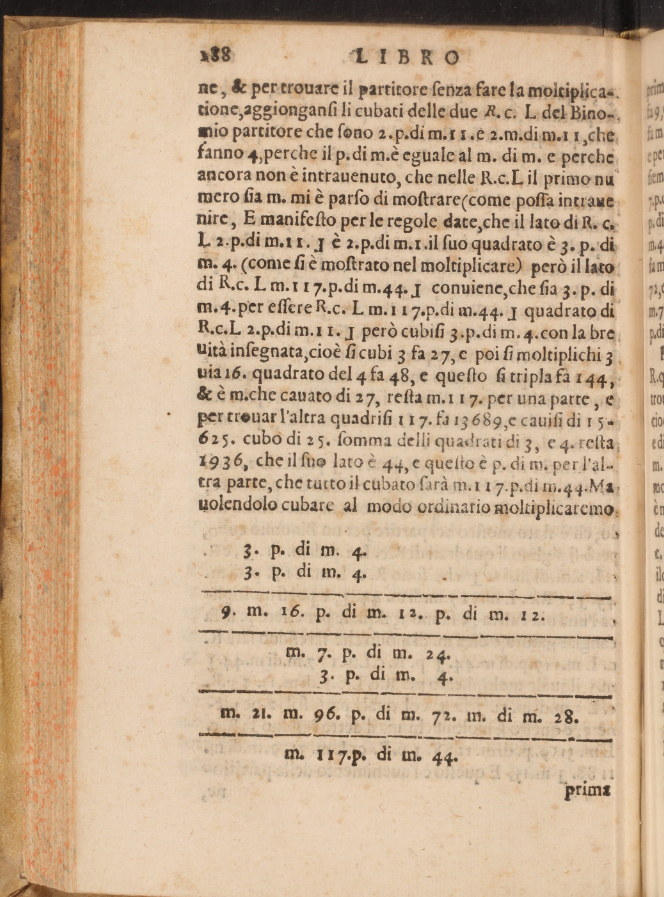
Figure 1: p. 188 of L’algebra by Rafael Bombelli. At this page, Bombelli demonstrated the steps to obtain \((3+4i)^{3}\). You can access a digital scanned copy here.
Bombelli’s discovery of the algebraic procedures for \(i\) was perhaps more on the experimental side. Nevertheless, he accurately provided the correct operational definitions for \(i\), which laid the foundation for further development of complex numbers.
Complex numbers’ definition and properties
Based on Bombelli’s discovery of imaginary numbers, we now define complex numbers as an ordered pair \((a,b)\) such that the addition and multiplication operations are defined as below:
\begin{align} (a_{1}, b_{1}) + (a_{2}, b_{2}) = (a_{1} + a_{2}, b_{1} + b_{2}) \\ (a_{1}, b_{1}) (a_{2}, b_{2}) = (a_{1} a_{2} - b_{1} b_{2}, a_{1} b_{2} + b_{1} a_{2}) \\ \end{align}Alternatively, if we rewrite \((a,b)\) as \(a + bi\), these follows directly form the definition of \(i^{2}=-1\) and the addition and multiplication defined for real numbers. Thus, similar to real numbers, the complex numbers form a field, which means the following properties hold for arbitrary complex numbers \(z_1\), \(z_2\), \(z_3\):
- Associativity: \(z_1 + (z_2 + z_3) = (z_1 + z_2) + z_3\) and \(z_{1} \cdot (z_{2} \cdot z_{3}) = (z_{1} \cdot z_{2}) \cdot z_{3}\).
- Commutativity: \(z_{1} + z_{2} = z_{2} + z_{1}\) and \(z_{1} \cdot z_{2} = z_{2} \cdot z_{1}\).
- Distributivity: \(z_{1} \cdot (z_{2} + z_{3}) = (z_{1} \cdot z_{2}) + (z_{1} \cdot z_{3})\).
- Additive and multiplicative identity: there exists \(0\) and \(1\) such that \(1 \cdot z_{1} = z_{1}\) and \(0 + z_{1} = z_{1}\).
- Additive and multiplicative inverse: for every \(z_{1}\), there exists \(-z_{1}\) and \(z_{1}^{-1}\) such that \(-z_{1} + z_{1} = 0\) and \(z_{1}^{-1} \cdot z_{1} = 1\).
These properties may seem a bit too abstract and without applications. However, it turns out that complex numbers can be used to succinctly represent 2D rotations.
Representing 2D rotations by complex numbers
The fact that complex numbers are merely an ordered pair of numbers admit another more geometric way of looking at this problem. Namely, the complex plane (originally proposed by Casper Wessel and Jean-Robert Argand).

Figure 2: Complex plane and complex number additions
The intuition behind this jump is simple. Because the two algebraic operations (addition and multiplication) of complex numbers are essentially inherited from real numbers, it is easy to map complex numbers to a 2D Cartesian plane. Thus, complex additions can be represented as vector additions on the complex plane (see Fig. 2).
Complex multiplications might seem a bit tricky at first. If we have \(z_{1} = a_{1} + b_{1} i\) and \(z_{2} = a_{2} + b_{2} i\), we can first multiply the two complex numbers out algebraically:
\begin{align} (a_{1} + \mathbf{i}b_{1}) (a_{2} + \mathbf{i}b_{2}) \\ = a_{1} a_{2} + \mathbf{i}a_{1} b_{2} + \mathbf{i}a_{2} b_{1} - b_{1} b_{2} \\ = (a_{1} a_{2} - b_{1} b_{2}) + \mathbf{i}(a_{1} b_{2} + a_{2} b_{1}) \end{align}
Figure 3: Complex plane and complex number multiplications.
To see how we can geometrically present complex multiplications, first notice that complex numbers hold the multiplicativity property of absolute values of real numbers as well:
\begin{align} \vert z_1 \vert \vert z_2 \vert = \vert z_1 z_2 \vert \end{align} \begin{align} (a^{2}_{1} + b^{2}_{1}) (a^{2}_{2} + b^{2}_{2}) = (a_1 a_2 - b_1 b_2)^{2} + (a_1 b_2 + a_2 b_1)^2 \end{align}The absolute values of complex numbers, on the complex plane, simply represents the squared distances from the origin to the points. In other words, the complex number we get after multiplying two complex numbers needs to have its distance to the origin equal to the product of the absolute values of the two complex numbers. Going back to Fig. 3: this means that the hypotenuse of the triangle we get from complex multiplication equals to the product of the hypotenuses of the two multiplicands.
Now that we know the length of the resulting complex number, how about the angle? After all, my claim is that complex numbers can be used to represent 2D rotations. It turns out that if we represent the \(a_{1}\), \(a_{2}\), \(b_{1}\) and \(b_{2}\) as trigonometric functions, we can solve for the angle between the product complex vector and the positive x-axis with ease. Let
\begin{align} a_{1} = A \cos{\theta} \\ b_{1} = A \sin{\theta} \\ a_{2} = B \cos{\phi} \\ b_{2} = B \sin{\phi} \end{align}where \(A = \sqrt{a^{2}_{1} + b^{2}_{1}}\) and \(B = \sqrt{a^{2}_{2} + b^{2}_{2}}\). Then, we have
\begin{align} a_{1} b_{2} + a_{2} b_{1} \\ = A \cos{\theta} \cdot B \sin{\phi} + B \cos{\phi} \cdot A \sin{\theta} \\ = AB \sin{(\theta + \phi)} \end{align}and
\begin{align} a_{1} a_{2} - b_{1} b_{2} \\ = A \cos{\theta} \cdot B \cos{\phi} - A \sin{\theta} \cdot B \sin{\phi} \\ = AB \cos{(\theta + \phi)} \end{align}Using our insights on the multiplicative properties of absolute values (and hypotenuses) before, we also know that
\begin{align} a_{1} b_{2} + a_{2} b_{1} = AB \sin{\psi} \\ a_{1} a_{2} - b_{1} b_{2} = AB \cos{\psi} \end{align}Thus, we have \(\psi = \theta + \phi\). This is saying that geometrically, when we multiply two complex numbers together, we are adding their angles together. In addition, for complex numbers with unitary absolute values, we can ignore the \(AB\) part. Thus, for unitary complex numbers as representations of 2D rotations, then multiplying together means concatenating their respective rotation operations.
Another view through matrices
Alternatively, we can represent complex numbers as 2-by-2 matrices. If we view complex numbers as an extension to the real numbers, then instead of a one-dimensional vector space, complex numbers form a two-dimensional vector space, with one possible basis as \((1, i)\) where \(i^{2} = -1\).
Also notice that
\begin{aligned} \begin{bmatrix} 0 & -1 \\ 1 & 0 \end{bmatrix}^2 = \begin{bmatrix} -1 & 0 \\ 0 & -1 \end{bmatrix} = -\mathbf{I} \end{aligned}where \(\mathbf{I}\) is the 2-by-2 identity matrix.
Thus, it follows that for a complex number \(a + b i\), we can represent it as
\begin{aligned} a + b\mathbf{i}\rightarrow \begin{bmatrix} a & -b \\ b & a \end{bmatrix} \end{aligned}The addition and multiplication operations follow the regular matrix addition and multiplication. The absolute value is defined as the determinant of the matrix. You can check whether such representation have the same properties as complex numbers (hint: they do!).
Following from our previous geometric interpretation, we can describe complex numbers \(a + bi\) in the form of \(A \cos{\theta} + A \sin{\theta} i\) where \(a = A \cos{\theta}\) and \(b = A \sin{\theta}\) and \(A\) being the length of the complex vector. Then, for unitary complex numbers, their matrix representations become
\begin{aligned} a + b\mathbf{i}\rightarrow \begin{bmatrix} \sin{\theta} & -\cos{\theta} \\ \cos{\theta} & \sin{\theta} \end{bmatrix} \end{aligned}Then, we have two complex numbers multiplied together as
\begin{align*} \begin{bmatrix} \sin{\theta} & -\cos{\theta} \\ \cos{\theta} & \sin{\theta} \end{bmatrix} \cdot \begin{bmatrix} \sin{\phi} & -\cos{\phi} \\ \cos{\phi} & \sin{\phi} \end{bmatrix} &= \begin{bmatrix} \cos{\theta} \cos{\phi} - \sin{\theta} \sin{\phi} & -\cos{\theta} \sin{\phi} - \sin{\theta} \cos{\phi} \\ \cos{\theta} \sin{\phi} + \sin{\theta} \cos{\phi} & \cos{\theta} \cos{\phi} - \sin{\theta} \sin{\phi} \end{bmatrix} \\ &= \begin{bmatrix} \sin{\theta + \phi} & -\cos{\theta + \phi} \\ \cos{\theta + \phi} & \sin{\theta + \phi} \end{bmatrix} \\ &= \begin{bmatrix} \sin{\psi} & -\cos{\psi} \\ \cos{\psi} & \sin{\psi} \end{bmatrix} \end{align*}Thus, we have \(\psi = \theta + \phi\), through another way of showing that multiplying complex numbers is equivalent to adding their rotation angles together.
Quaternions for 3D rotations
Complex numbers form an algebra of pairs of numbers. So a natural question is: does there exist an algebra for 3 numbers? Or 4 numbers? Or even more? It turns out that there exists only such algebra of dimension 1, 2 and 4, corresponding to the real numbers, complex numbers and quaternions respectively.
Hamilton’s obsession
William Hamilton was looking for a way to extend the algebra of complex numbers to triplets of numbers. He already understood that complex numbers are essentially the extension of algebra of reals to pairs of numbers, and he is obsessed with finding an algebra that works with triplets of numbers. Legend has it, on August 5th, 1865, Hamilton was walking along the Royal Canal in Dublin towards the Royal Irish Academy. When he walked past Broome bridge, Hamilton in a flash of genius realized that instead of triplets, four numbers can be used to construct an algebra, with three imaginary numbers follow the following properties:
\begin{align*} \mathbf{i}1 = 1 \mathbf{i}= \mathbf{i}, \qquad \mathbf{j}1 = 1\mathbf{j} = \mathbf{j}, \qquad \mathbf{k}1 = 1\mathbf{k} = \mathbf{k} \\ \mathbf{i}^{2} = \mathbf{j}^{2} = \mathbf{k}^{2} = \mathbf{ijk} = -1, \qquad \mathbf{ij}=\mathbf{k}, \qquad \mathbf{ji}=-\mathbf{k} \\ \end{align*}With these properties, the three imaginary numbers have a cyclic structure, namely the product of any two distinct elements equal to the other one, and the sign is determined by the direction of the product:
\begin{align*} \mathbf{jk} = \mathbf{i}, \quad \mathbf{kj} = -\mathbf{i}\\ \mathbf{ki}= \mathbf{j}, \quad \mathbf{ik} = -\mathbf{j} \end{align*}The rules can be represented by a multiplication table:
| x | 1 | \(\mathbf{i}\) | \(\mathbf{j}\) | \(\mathbf{k}\) |
| \(\mathbf{1}\) | 1 | \(\mathbf{i}\) | \(\mathbf{j}\) | \(\mathbf{k}\) |
| \(\mathbf{i}\) | \(\mathbf{i}\) | -1 | \(\mathbf{k}\) | -\(\mathbf{j}\) |
| \(\mathbf{j}\) | \(\mathbf{j}\) | -\(\mathbf{k}\) | -1 | \(\mathbf{i}\) |
| \(\mathbf{k}\) | \(\mathbf{k}\) | \(\mathbf{j}\) | -\(\mathbf{i}\) | -1 |
The resulting numbers, which consists of a real part and three imaginary numbers, are called quaternions: \[ q = a + b\mathbf{i}+ c\mathbf{j} + d\mathbf{k} \] Quaternion sums have the exact same properties as real number additions: you can simply perform element-wise addition. Namely,
- Associativity: \(q_1 + q_2 = q_2 + q_1\)
- Commutativity: \(q_{1} + (q_{2} + q_{3}) = (q_{1} + q_{2}) + q_{3}\)
- Additive identity: \(q + (-q) = 0\)
- Additive inverse: \(q + 0 = q\)
For multiplication, quaternions follow the same distributive law used in complex numbers. In other words, for \(q_{1}=a_{1}+b_{1}\mathbf{i}+c_{1}\mathbf{j}+d_{1}\mathbf{k}\) and \(q_{2}=a_{2}+b_{2}\mathbf{i}+c_{2}\mathbf{j}+d_{2}\mathbf{k}\), we have
\begin{align*} q_{1} \cdot q_{2} =& a_{1} a_{2}+a_{1} b_{2} \mathbf{i}+a_{1} c_{2} \mathbf{j}+a_{1} d_{2} \mathbf{k} \\ &+b_{1} a_{2} \mathbf{i}+b_{1} b_{2} \mathbf{i}^{2}+b_{1} c_{2} \mathbf{i} \mathbf{j}+b_{1} d_{2} \mathbf{ik} \\ &+c_{1} a_{2} \mathbf{j}+c_{1} b_{2} \mathbf{j i}+c_{1} c_{2} \mathbf{j}^{2}+c_{1} d_{2} \mathbf{j k} \\ &+d_{1} a_{2} \mathbf{k}+d_{1} b_{2} \mathbf{k i}+d_{1} c_{2} \mathbf{k j}+d_{1} d_{2} \mathbf{k}^{2} \\ =& a_{1} a_{2}-b_{1} b_{2}-c_{1} c_{2}-d_{1} d_{2} \\ &+\left(a_{1} b_{2}+b_{1} a_{2}+c_{1} d_{2}-d_{1} c_{2}\right) \mathbf{i} \\ &+\left(a_{1} c_{2}-b_{1} d_{2}+c_{1} a_{2}+d_{1} b_{2}\right) \mathbf{j} \\ &+\left(a_{1} d_{2}+b_{1} c_{2}-c_{1} b_{2}+d_{1} a_{2}\right) \mathbf{k} \end{align*}A more succinct way to write this is to treat the real number as the scalar part of the quaternion and the three imaginary numbers as the vector part of the quaternion. Let \(q_{1} = (r_{1}, \vec{v}_{1})\) and \(q_{2} = (r_{2}, \vec{v}_{2})\). The multiplication can then be rewritten as
\begin{align} \left(r_{1}, \vec{v}_{1}\right)\left(r_{2}, \vec{v}_{2}\right)=\left(r_{1} r_{2}-\vec{v}_{1} \cdot \vec{v}_{2}, r_{1} \vec{v}_{2}+r_{2} \vec{v}_{1}+\vec{v}_{1} \times \vec{v}_{2}\right) \label{eq:quat-product-vec} \tag{1} \end{align}with \(\cdot\) representing the standard dot product and \(\times\) representing the standard cross product. In fact, Hamilton’s quaternion products are the places where vector dot and cross products appear for the first time in history.
Similar to complex numbers, we can also represent quaternions as matrices:
\begin{align} \begin{bmatrix} a + d\mathbf{i} & -b - c\mathbf{i} \\ b - c\mathbf{i} & a - d\mathbf{i} \\ \end{bmatrix} = a + b \mathbf{i} + c \mathbf{j} + d \mathbf{k} \end{align}You can check for yourselves that the algebraic rules still hold.
In addition, quaternions also have conjugates. The conjugate \(\bar{q}\) of \(q=a+b\mathbf{i}+c\mathbf{j}+d\mathbf{k}\) equals to \(a-b\mathbf{i}-c\mathbf{j}-d\mathbf{k}\). And the norm \(|q|\) of the quaternion \(q\) equals to \(q\bar{q} = a^{2} + b^{2} + c^{2} + d^{2}\).
Quaternion multiplication is not commutative. However, this is more of a boon than a bane. This has made quaternion algebra be of a division algebra, where the quotient of an element of the algebra by any other nonnull element always exists, and that the product of two elements must vanish if and only if one of the factors is the null element. The non-commutativity of quaternion algebra has precisely allowed this to happen. If the multiplication rules are commutative, say \(\mathbf{ij} = \mathbf{ji}= \mathbf{k}\), then product of nonnull elements such as \(q_{1} = \mathbf{i}+ \mathbf{j}\) and \(q_{2} = -\mathbf{i}+ \mathbf{j}\) will vanish. With this property, we can see that the inverse of a quaternion \(q\) can be expressed as: \[ q^{-1} = \frac{\bar{q}}{|q|^{2}} =\frac{1}{a^{2} + b^{2} + c^{2} + d^{2}}(a - b\mathbf{i}- c\mathbf{j} - d\mathbf{k}) \]
With these properties nailed down, we are now ready to proceed towards using quaternions to represent 3D rotations.
Towards 3D rotations: the algebra
What is a rotation? Generally speaking, rotations transform a vector to a new position without changing its norm and keeping its tail fixed. So if quaternions are to represent 3D rotations, whatever operations they perform should not affect the norm of the resulting vector, and that the origin should stay fixed. Let’s keep these two requirements in mind, as they will be useful to see whether the operations we find actually represent 3D rotations.
The first obstacle we need to overcome is how to represent the object under 3D rotations. After all, what we have are quaternions, which have four numbers instead of three. To resolve this, we use the most simple solution: we force the scalar part of the quaternion to be zero, and only look at the vector part of the quaternion (which is why that part is called the vector). We define such quaternions \(q = b\mathbf{i}+ c\mathbf{j} + d\mathbf{k}\) as pure imaginary quaternions, and the three-dimensional space as \(\mathbb{R}^{3}\).
Now, we have the object under rotations (pure imaginary quaternions), we need to define the operators for rotations. One may first attempt to simply use quaternion multiplications to represent rotations. However, doing so will not keep the pure imaginary quaternions as pure imaginary. We can see it from Eq. \ref{eq:quat-product-vec} that the scalar part of the product quaternion is zero only if one of them have a scalar part equals to zero and that the vector parts are orthogonal to each other.
Instead, we use an operation called conjugation. The conjugation of a quaternion \(q\) by another quaternion \(t\) is: \[ q \rightarrow t q t^{-1} \] Second, we will force \(|t|=1\), similar to the case of complex numbers.
With conjugation, if \(q\) is a pure imaginary quaternion, \(t q t^{-1}\) is also pure imaginary as long as \(t\) is a unit quaternion. To see why, first we will use a parameterization similar to what we did for complex numbers. Namely, we will introduce \(\cos{\theta}\) and \(\sin{\theta}\) to represent unit quaternions: \[ t = \cos{\theta} + \sin{\theta} u \] where \(|\vec{u}| = 1\). This is essentially saying that we can separate a quaternion into two quaternions, where the first one represents the scalar part of the original quaternion, and the second one represents the vector part of the quaternion. It is trivial to see that \(|t|=1\) as expected.
In addition, we have \(t^{-1} = \cos{\theta} - \sin{\theta} \vec{u}\) (you can check that \(t t^{-1} = 1\)) So we have:
\begin{align*} t q t^{-1} &= (\cos{\theta} + \sin{\theta} u) q (\cos{\theta} - \sin{\theta} u) \\ &= (\cos{\theta}q + \sin{\theta} uq) (\cos{\theta} - \sin{\theta} u) \\ &= q \cos^{2}{\theta} + \sin{\theta} \cos{\theta} uq - \cos{\theta} \sin{\theta} qu - \sin^{2}\theta uqu \end{align*}Let \(u = (0, \vec{b_{1}})\) and \(v = (0, \vec{b_{2}})\).
Since \(q\) is already a pure imaginary quaternion, we only need to look at the \(uq\), \(qu\) and \(uqu\) terms. Note that \(uq = (- \vec{b_{1}} \cdot \vec{b_{2}}, \vec{b_{1}} \times \vec{b_{2}})\) and that \(qu = (- \vec{b_{2}} \cdot \vec{b_{1}}, \vec{b_{2}} \times \vec{b_{1}})\) So \[ -uq + qu = (0, 2\vec{b_{2}} \times \vec{b_{1}}) \] and it’s clear that the scalar part equals to zero.
Now, let’s look at the term containing \(uqu\). For simplicity, let \(uq = (- \vec{b_{1}} \cdot \vec{b_{2}}, \vec{b_{1}} \times \vec{b_{2}}) = (A, \vec{B})\). Then we have \[ uqu = (-\vec{B} \cdot \vec{b_{1}}, A \vec{b_{1}} + \vec{B} \times \vec{b_{1}}) \] Note that \(-\vec{B} \cdot \vec{b_{1}} = - \vec{b_{1}} \times \vec{b_{2}} \cdot \vec{b_{1}}\), which equals to zero, because \(\vec{b_{1}} \times \vec{b_{2}}\) is perpendicular to \(\vec{b_{1}}\).
Thus, we have \(t q t^{-1}\) a purely imaginary quaternion. And we now are ready to prove the following theorem about conjugation:
Theorem: Given \(t = \cos{\theta} + \sin{\theta} u\), where \(u\) is a unit vector in \(\mathbb{R}^{3}\), then conjugation by \(t\) rotates \(\mathbb{R}^{3}\) through angle \(2\theta\) about axis \(u\).
Proof: First, notice that the line formed by multiples of \(u\) is fixed:
\begin{align*} t u t^{-1} &= (\cos{\theta} + \sin{\theta} u) u (\cos{\theta} - \sin{\theta}u) \\ &= (\cos{\theta} u + \sin{\theta} u^{2}) (\cos{\theta} - \sin{\theta}u) \\ \end{align*}Note that \(u^{2} = -u \cdot u = - |u|^{2} = -1\), so we have
\begin{align*} t u t^{-1} &= (\cos{\theta} u - \sin{\theta}) (\cos{\theta} - \sin{\theta} u) \\ &= (\cos^{2}{\theta} + \sin^{2}{\theta}) u - \cos{\theta} \sin{\theta} u^{2} - \sin{\theta} \cos{\theta} \\ &= u \end{align*}
Figure 4: The construction of vectors \(v\) and \(w\) from \(u\).
Then, we need to check whether the plane orthogonal to the line \(u\) is rotated. Let \(v\) be a \(\mathbb{R}^{3}\) vector orthogonal to \(u\), and let \(w = u \times v = uv\). The plane spanned by \(v\) and \(w\) are therefore orthogonal to \(u\) (see Fig. 4). We now show that the two bases \(v\) and \(w\) gets rotated by \(2\theta\).
Consider \(t v t^{-1}\):
\begin{align*} t v t^{-1} &= (\cos{\theta} + \sin{\theta} u) v (\cos{\theta} - \sin{\theta}u) \\ &= (\cos{\theta} v + \sin{\theta} uv) (\cos{\theta} - \sin{\theta}u) \\ &= \cos^{2}{\theta} v - \sin{\theta} \cos{\theta} vu + \sin{\theta} \cos{\theta} uv - \sin^{2}{\theta} uvu \\ &= \cos^{2}{\theta} v + 2 \sin{\theta} \cos{\theta} uv + \sin^{2}{\theta} u^{2} v \quad \text{because $vu = -uv$} \\ &= (\cos^{2}{\theta} - \sin^{2}{\theta}) v + 2\sin{\theta} \cos{\theta}w \quad \text{because $u^{2}=-1$ and $uv = w$} \\ &= \cos{2\theta} v + \sin{2\theta} w \end{align*}Similarly, for \(t w t^{-1}\):
\begin{align*} t w t^{-1} &= (\cos{\theta} + \sin{\theta} u) w (\cos{\theta} - \sin{\theta}u) \\ &= (\cos{\theta}w + \sin{\theta} u w) (\cos{\theta} - \sin{\theta}u) \\ &= \cos^{2}{\theta} w - \cos{\theta} \sin{\theta} wu + \sin{\theta} \cos{\theta} uw - \sin^{2}{\theta} uwu \\ &= \cos^{2}{\theta} w - 2\cos{\theta} \sin{\theta} wu - \sin^{2}{\theta} uwu \\ &= (\cos^{2}{\theta} - \sin^{2}{\theta} )w - 2\cos{\theta} \sin{\theta} v \\ &= \cos{2\theta} w - \sin{2\theta}v \end{align*}It is easy to see that \(t v t^{-1}\) and \(t w t^{-1}\) rotate \(v\) and \(w\) by \(2 \theta\), as required (Fig. 5). Thus, we have proved our theorem.

Figure 5: Rotation of \(v\) and \(w\) on the plane \(vw\) orthogonal to the vector \(u\). Using elementary trignometry, we can see that the rotated \(v^{\prime}=\cos{2\theta} v + \sin{2\theta} w\) and \(w^{\prime}=\cos{2\theta} w - \sin{2\theta}v\), exactly what we derived from quaternion conjugation.
To summarize, every rotation in \(\mathbb{R}^{3}\) given by an axis \(u\) and an angle of rotation \(\alpha\) is the result of conjugation by the unit quaternion \[ t = \cos{\frac{\alpha}{2}} + u \sin{\frac{\alpha}{2}} \]
Note that \(-t\) induces the same rotation as \(t\), which intuitively makes sense, considering it is simply a rotation about an axis in the opposite direction with the negative of the angle.
Towards 3D rotations: the geometry
It’s nice and all that quaternions can be shown to algebraically allow us to represent 3D rotations. However, the choice of the parametrization of quaternions with \(\cos{\theta}\) and \(\sin{\theta}\) seems a bit too arbitrary. It turns out that there is a geometric argument for the quaternion algebra, and that it was discovered by a French banker and mathematician named Olinde Rodrigues in 1840, five years before Hamilton’s epiphany about quaternions!
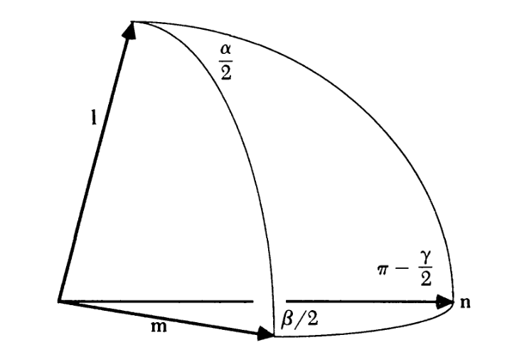
Figure 6: Rotate angle \(\beta\) around \(m\), then rotate \(\alpha\) around \(l\), equals to rotating angle \(\gamma\) around \(n\). (source: Altmann, Simon L. “Hamilton, Rodrigues, and the quaternion scandal.” Mathematics Magazine 62.5 (1989): 291-308.)
Rodrigues discovered that if one rotates angle \(\beta\) around \(m\), then rotates \(\alpha\) around \(l\), the resulting rotation is a rotation of angle \(\gamma\) around \(l\), which follows the following equations:
\begin{align*} \cos \frac{\gamma}{2} &= \cos \frac{\alpha}{2} \cos \frac{\beta}{2}-\sin \frac{\alpha}{2} \sin \frac{\beta}{2} l \cdot \mathrm{m} \\ \sin \frac{\gamma}{2} \mathbf{n} &=\sin \frac{\alpha}{2} \cos \frac{\beta}{2} \mathbf{l}+\cos \frac{\alpha}{2} \sin \frac{\beta}{2} \mathbf{m}+\sin \frac{\alpha}{2} \sin \frac{\beta}{2} l \times \mathbf{m} . \end{align*}Notice how the equation above is basically the quaternion product \(q_{1} q_{2}\) with \(q_{1} = (\cos{\frac{\alpha}{2}}, \sin{\frac{\alpha}{2}} \mathbf{l})\) and \(q_{2}= (\cos{\frac{\beta}{2}}, \sin{\frac{\beta}{2}} \mathbf{m})\).
Conclusion and references
Quaternions and complex numbers are interesting because they have clear algebraic roots, and yet they also have deep geometric interpretations. Before writing this post, I’ve been treating quaternion algebra as a black box that one just need to memorize how to use. Hopefully this article will also help you if you are not sure why quaternions work the way they do.
References that I studied when writing this blog post:
- Stillwell, John. Naive lie theory. Springer Science & Business Media, 2008.
- Altmann, Simon L. “Hamilton, Rodrigues, and the quaternion scandal.” Mathematics Magazine 62.5 (1989): 291-308.
- Wikipedia page on quaternions.
- Wikipedia page on Olinde Rodrigues.
- Wikipedia page on William Rowan Hamilton.
In particular, the proofs for quaternion conjugation come from Stillwell (with some modifications), which is an excellent textbook on Lie groups.