Use Gröbner Bases To Solve Polynomial Equations
Update 1 (2023/04/26): See Hacker News discussion here.
I’ve seen Gröbner bases in many research papers 1 , 2. As an excuse to learn more about them, I write this article down to serve both as a note for me as well as a tutorial for interested readers to get a brief glimpse of the power of Gröbner bases.
To fully explore Gröbner bases and related, we need to involve a multitude of different topics in algebraic geometry; and to be frank, I am not currently capable of doing so. Hence, I will exclusively focus on the topic of using Gröbner Bases to solve polynomial equations, which is interesting and useful to many. I will accompany the discussions with short code snippets in Python using the SymPy package. You can also find code snippets used in this post in my code repo here.
This article relies heavily in terms of examples and definitions on the fantastic textbook Ideals, Varieties and Algorithms: An Introduction to Computational Algebraic Geometry and Commutative Algebra by David A. Cox, John Little and Donal O’Shea3. Interested readers should refer to it for more detailed exposition on this topic. In addition, lecture handouts by Judy Holdener at CMU are very helpful4. I list additional references at the end of this post.
A Motivational Problem
First, let’s motivate the study of Gröbner bases through an example of solving a system of linear equations. Consider the following set of linear equations
\begin{align} 2x_{1} + 3 x_{2} - x_{3} &= 0 \\ x_{1} + x_{2} - 1 &= 0 \\ x_{1} + x_{3} - 3 &= 0 \end{align}which can be written in the matrix form
\begin{align} \begin{pmatrix} 2 & 3 & -1 & 0 \\ 1 & 1 & 0 & 1 \\ 1 & 0 & 1 & 3 \end{pmatrix}. \end{align}By performing Gaussian Elimination, we arrive at the reduced row echelon form
\begin{align} \begin{pmatrix} 1 & 0 & 1 & 3 \\ 0 & 1 & -1 & -2 \\ 0 & 0 & 0 & 0 \end{pmatrix}. \end{align}You can check this yourself by running the following Python code using SymPy:
import sympy as sp
def gaussian_elimination(M):
    return M.rref()[0]

gaussian_elimination(sp.Matrix([[2, 3, -1, 0],
                                [1, 1, 0, 1],
                                [1, 0, 1, 3]]))
The results should look like this:
Matrix([[1, 0, 1, 3], [0, 1, -1, -2], [0, 0, 0, 0]])
From the above, we can see that the solution to the system is
\begin{align} x_{1} = -t + 3, \\ x_{2} = t - 2, \\ x_{3} = t. \end{align}which is equivalent to a line in \(\mathbb{R}^{3}\).
Now, can we do something similar to a system of polynomial equations? In other words, we want to develop a method to determine the solution to
\begin{align} f_{1}(x_{1}, x_{2}, \ldots, x_{n}) = f_{2}(x_{1}, x_{2}, \ldots, x_{n}) = \cdots = f_{s}(x_{1}, x_{2}, \ldots, x_{n}) = 0. \end{align}The method of Gröbner bases allows us to do so.
A Taste of Gröbner Bases
I will start with a concrete example of using Gröbner Bases to solve a system of polynomial equations. Words and phrases in bold are new concepts which I will define later.
Consider the following system of equations:
\begin{align} x^{2} + y + z = 1, \\ x + y^{2} + z = 1, \\ x + y + z^{2} = 1. \end{align}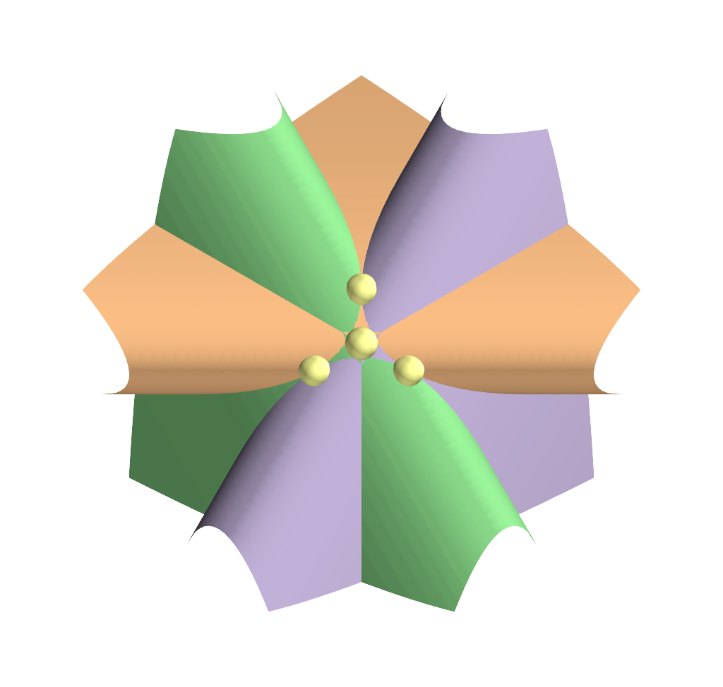
Figure 1: Visualization of the system of polynomial equations above. The three equations are represent as the three surfaces, and the solutions are represented as spheres. The four visible spheres represent \((1,0,0)\), \((0,1,0)\), \((0,0,1)\) and \((-1+\sqrt{2},-1+\sqrt{2},-1+\sqrt{2})\). There is one more occluded solution at the back, corresponding to \((-1 - \sqrt{2}, -1 - \sqrt{2}, -1 - \sqrt{2})\).
We first define the ideal
\begin{align} I = \langle x^{2} + y + z - 1, x + y^{2} + z - 1, x + y + z^{2} - 1 \rangle. \end{align}where the angle brackets represent a set of polynomials following
\begin{align} \left\langle f_1, \ldots, f_s\right\rangle=\left\{\sum_{i=1}^s h_i f_i \mid h_1, \ldots, h_s \in k\left[x_1, \ldots, x_n\right]\right\}. \end{align}Right now treat this ideal roughly as the set of polynomials of which the solutions to \(x\), \(y\) and \(z\) satisfies the original polynomial system. The Gröbner bases for this ideal \(I\) with respect to lex order is the following:
\begin{align} g_{1} = x + y + z^{2} - 1, \\ g_{2} = y^{2} - y - z^{2} + z, \\ g_{3} = 2yz^{2} + z^{4} - z^{2}, \\ g_{4} = z^{6} - 4z^{4} + 4z^{3} - z^{2}. \\ \end{align}Note that \(g(4)\) contains only \(z\), and
\begin{align} g(4) = z^{6} - 4z^{4} + 4z^{3} - z^{2} = z^{2} (z - 1)^{2} (z^{2} + 2z - 1), \end{align}which becomes zero when \(z = 0, 1, -1 + \sqrt{2}, -1 - \sqrt{2}\). Substituting them back to \(g_{2} = 0\) and \(g_{3} = 0\), we can determine \(y = 1, 0, -1 + \sqrt{2}, -1 - \sqrt{2}\). Then using \(g_{1}\), we can get the corresponding values for \(x\), which leads to the following five possible solutions to the original system:
\begin{align} (1, 0, 0), \\ (0, 1, 0), \\ (0, 0, 1), \\ (-1+\sqrt{2},-1+\sqrt{2},-1+\sqrt{2}), \\ (-1-\sqrt{2},-1-\sqrt{2},-1-\sqrt{2}), \\ \end{align}Notice how the existence of \(g(4)\), a polynomial with only one variable \(z\), enables us to solve for all variables through back-substitution. To understand how this process works, we need to answer the following two questions:
- What is the relationship of the ideal with respect to the original system of equations?
- What are Gröbner bases?
- How do Gröbner bases help us solve polynomial systems?
Now we will make an attempt to answer these three questions.
Background
Unfortunately we need to go over a few definitions so that we have a common ground for discussing Gröbner bases. Concepts like polynomials should be familiar, but we need some more definitions in order to discuss them in a precise manner. We will see relevant SymPy code as well to play around with some of the concepts.
Some Concepts from Abstract Algebra
A field is a set \(k\) with two operations defined: \(+\) and \(\cdot\), with the following properties:
- Associativity: \((a+ b) + c = a + (b + c)\) and \((a \cdot b) \cdot c = a \cdot (b \cdot c)\),
- Commutativity: \(a + b = b + a\) and \(a \cdot b = b \cdot a\),
- Distributivity: \(a \cdot (b + c) = a \cdot b + a \cdot c\),
- Identities: there exist \(0\) and \(1\) in \(k\) such that \(a + 0 = 1 \cdot a = a\),
- Additive Inverses: for each \(a\), there exists \(b\) such that \(a + b = 0\),
- Multiplicative Inverses: for each \(a \neq 0\), a \(c\) exists in \(k\) such that \(a \cdot c = 1\).
Examples of fields include \(\mathbb{Q}\), \(\mathbb{R}\) and \(\mathbb{C}\).
Monomials and Polynomials
Assume \(x_{1}, \ldots, x_{n}\) are variables. A monomial in \(x_{1}, \ldots, x_{n}\) is a product of the form \(x^{\alpha_{1}}_{1} \cdot x^{\alpha_{2}}_{2} \cdots x^{\alpha_{3}}_{3}\). The total degree of a monomial is \(\sum_{1}^{n} \alpha_{i}\). Alternatively, we can use a vector notation, with \(\alpha = (\alpha_{1}, \ldots, \alpha{n})\) and
\begin{align} x^{\alpha} =x^{\alpha_{1}}_{1} \cdot x^{\alpha_{2}}_{2} \cdots x^{\alpha_{3}}_{3}. \end{align}A polynomial \(f\) is a finite collection of monomials with coefficients in field \(k\), in the form of
\begin{align} f = \sum_{\alpha \in \mathcal{A}} a_{\alpha} x^{\alpha} \end{align}where \(\mathcal{A}\) is a finite set containing n-tuples, \(a_{\alpha}\) is the coefficient of the monomial term \(x^{\alpha}\). \(a_{\alpha} x^{\alpha}\) is a term of the polynomial if \(a_{\alpha} \neq 0\). Denote the set of all polynomials in \(x_{1}, \ldots, x_{n}\) with coefficients in field \(k\) as \(k[x_{1}, \ldots, x_{n}]\). The total degree of a polynomial is the maximum \(\| \alpha \|\) of all terms in the polynomial.
In SymPy, polynomials are created by constructing expressions using predefined symbols:
from sympy import poly
from sympy.abc import x, y, z

# a single variable polynomial
A = poly(x**2 + 2*x + 1)

# a 3-variable polynomial
B = poly(x**2 + y + z)
A and B should be Poly(x**2 + 2*x + 1, x, domain='ZZ') and Poly(x**2 + y + z, x, y, z, domain='ZZ') respectively.
The parameter domain represents the domain in which coefficients of the polynomial reside, in this case integers (ZZ).
Monomial Ordering
An important concept regarding polynomials is that of ordering. Let’s observe the Gaussian elimination process. During row reduction, we are working systematically to reduce the leftmost entry to zero for each row, with the first nonzero entry in the row as the leading term. For polynomials, monomial ordering formalizes this concept. A monomial ordering \(>\) on the polynomial \(k[x_{1}, \ldots, x_{n}]\) is a relation on \(\mathbb{Z}^{n}_{\geq 0}\) (the set of exponents of the monomials as n-tuples) such that
- for every pair of \(x^{\alpha}\) and \(x^{\beta}\), exactly one of the three statements is true: \(\alpha > \beta\), \(\alpha = \beta\) or \(\beta > \alpha\),
- if \(\alpha > \beta\), and \(\gamma \in \mathbb{Z}^{n}_{\geq 0}\), then \(\alpha + \gamma > \beta + \gamma\),
- \(>\) is a well-ordering on \(\mathbb{Z}^{n}_{\geq 0}\) (equivalent to saying every non-empty subset of \(\mathbb{Z}^{n}_{\geq 0}\) has a smallest element under \(>\)).
We say \(x^{\alpha} > x^{\beta}\) if \(\alpha > \beta\).
The simplest example of monomial ordering is the lexicographic order \(>_{lex}\). In this order, \(\alpha >_{lex} \beta\) if the leftmost non-zero entry of \(\alpha - \beta\) is positive. So \(x_{1} >_{lex} x_{2} >_{lex} x_{3} \cdots >_{lex} x_{n}\). You can prove that this order is a proper monomial ordering. Note that given a set of \(n\) variables, there are actually \(n!\) lexicographic orders. However by convention we adopt \(x_{1} >_{lex} x_{2} >_{lex} x_{3} \cdots >_{lex} x_{n}\). If we are using \(x\), \(y\), and \(z\) as varialbes, we assume \(x > y > z\).
Here are some examples of comparing monomials using lexicographic orders:
- \(x^{3} >_{lex} x^{2}y^{4}\)
- \(x^{2}yz >_{lex} xyz\)
- \(xy^{2}z >_{lex} z^{2}\)
Another potential monomial ordering is the graded lexicographic order \(>_{grlex}\). By graded, it means we need to consider the total degrees of the monomial terms. Let \(\alpha, \beta \in \mathbb{Z}^{n}_{\geq 0}\). \(\alpha >_{grlex} \beta\) if
\begin{align} \| \alpha \| > \| \beta \|, \quad \text{or} \quad \| \alpha \| = \| \beta \| and \alpha >_{lex} \beta \end{align}Here are the same examples of comparisons using graded lexicographic order:
- \(x^{2}y^{4} >_{grlex} x^{3}\)
- \(x^{2}yz >_{grlex} xyz\)
- \(xy^{2}z >_{grlex} z^{2}\)
Given a monomial order \(>\) and a polynomial \(f = \sum_{\alpha} a_{\alpha} x^{\alpha}\) in \(k[x_{1}, \ldots, x_{n}]\), we define the following:
The multidegree of f is:
\begin{align} \text{multideg}(f) = \max(\alpha \in \mathbb{Z}^{n}_{\geq 0} \mid a_{\alpha} \neq 0) \end{align}The leading coefficient of f is
\begin{align} \text{LC}(f) = a_{\text{multideg}(f)} \in k \end{align}The leading monomial of f is
\begin{align} \text{LM}(f) = x^{\text{multideg}(f)} \end{align}The leading term of f is
\begin{align} \text{LT}(f) = \text{LC} \cdot \text{LM} (f) \end{align}
Note that since the \(\max\) function depends on the monomial order \(>\) we use, all definitions above depends on the choice of the monomial order.
In SymPy, we have a few handy functions to get these properties of polynomials:
from sympy import poly, LC, LM, LT
from sympy.abc import x, y, z

# a single variable polynomial
f = poly(4*x**2*y + 2*x*y*z + z**2)

# leading coefficient
# note: x,y,z represent the monomial ordering used
# you can also use: f.LC(order='lex')
print(f"LC(f): {LC(f, x, y, z)}")

# leading monomial
print(f"LM(f): {LM(f, x, y, z)}")

# leading term
print(f"LT(f): {LT(f, x, y, z)}")
Running the above should give you:
LC(f): 4
LM(f): x**2*y
LT(f): 4*x**2*y
With the definitions, we are now geared up to dive deeper into the topics of Gröbner bases and polynomials.
Ideals and Solutions to Systems of Polynomials
We now try to answer Question 1 we proposed at the end of Section A Taste of Gröbner Bases. In particular, we define what exactly are the solutions to a system of polynomials, and how ideals relate to them.
Affine Varieties
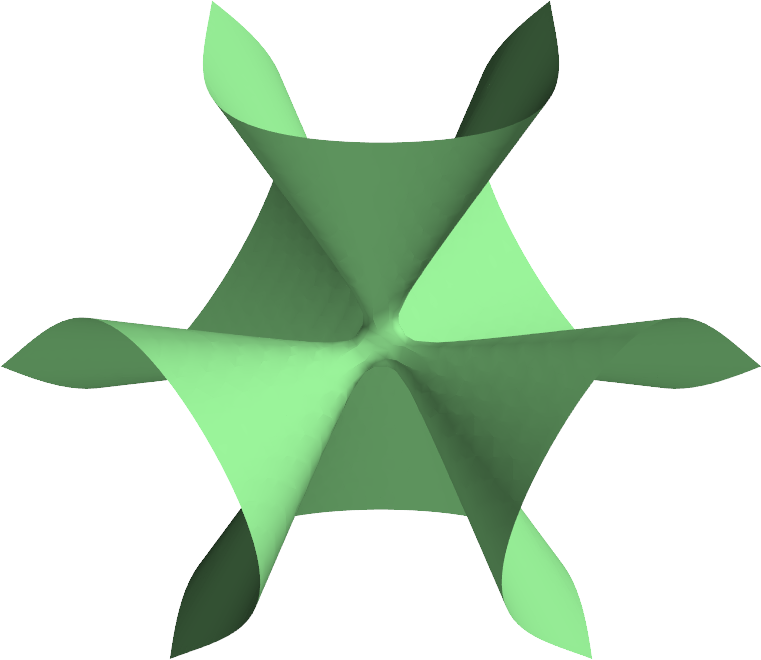
Figure 2: Visualization of the Clebsch surface. Refer to here for more information about this unique cubic surface.
An affine variety is the set of all solutions to a system of polynomials. Specifically,
\begin{align} \mathbf{V}(f_{1}, \ldots, f_{s}) = \{ (a_{1}, \ldots, a_{n}) \in k^{n} \mid f_{i} (a_{1}, \ldots, a_{n}) = 0, 1 \leq i \leq s \}, \end{align}where \(f_{1}, \ldots, f_{s}\) are polynomials in \(k[x_{1}, \ldots, x_{n}]\).
An example visualization of a variety, called the Clebsch surface, is shown in Fig. 2, where the variety is
\begin{gather} \mathbf{V}(81 (x^3 + y^3 + z^3) – 189 (x^2 y + x^2 z + x y^2 + x z^2 + y^2 z + y z^2) \\ + 54 xyz + 26(xy + xz + yz) – 9(x^2 + y^2 + z^2) – 9(x + y + z) + 1). \end{gather}Ideals
An ideal is a subset of polynomials \(I \subset k[x_{1}, \ldots, x_{n}]\) if
- \(0 \in I\),
- If \(f, g \in I\), then \(f + g \in I\),
- If \(f \in I\), and \(h \in k[x_{1}, \ldots, x_{n}]\) then \(hf \in I\).
Ideal is a very natural concept for polynomials. Consider
\begin{align} \langle f_{1}, \ldots, f_{s} \rangle = \left\{ \sum_{i=1}^{s} h_{i} f_{i} \mid h_{1}, \ldots, h_{s} \in k[x_{1}, \ldots, x_{n}] \right\} \end{align}which is a set of polynomials formed by a finite set of polynomials \(f_{1}\) to \(f_{s}\) multiplying with other polynomials \(h_{i}\). This set \(\langle f_{1}, \ldots, f_{s} \rangle\) is actually an ideal, which you can show easily by testing out the three conditions. In addition, if an ideal can be expressed in the form of \(\langle f_{1}, \ldots, f_{s} \rangle\), we say this ideal is finitely generated, and that the set \(f_{1}, \dots, f_{s}\) is a basis of ideal.
It turns out that every ideal of \(k\left[ x_{1}, \ldots, x_{n} \right]\) is finitely generated:
Theorem 1 (Hilbert Basis Theorem): Every ideal \(I \subseteq k\left[ x_{1}, \ldots, x_{n} \right]\) has a finite generating set \(g_{1}, \ldots, g_{t} \in I\) such that \(I = \langle g_{1}, \ldots, g_{t} \rangle\).
The proof of Theorem 1 requires the usage of the division algorithm, which will complicate the narrative quite a bit. Interested readers can refer to Section 5, Chapter 2 of 3.
Ideals relate closely to systems of polynomial equations. Consider the system
\begin{align} f_{1} = f_{2} = \ldots = f_{s} = 0. \end{align}It’s easy to see that
\begin{align} h_{1} f_{1} + h_{2} f_{2} + \ldots + h_{s} f_{s} = 0 \end{align}for polynomials \(h_{i}\). And by definition, \(h_{1} f_{1} + h_{2} f_{2} + \ldots + h_{s} f_{s}\) is a member of the ideal \(\langle f_{1}, \ldots, f_{s} \rangle\). Naturally, We can define the affine variety induced by an ideal \(I\) as:
\begin{align} \mathbf{V}(I)=\left\{\left(a_1, \ldots, a_n\right) \in k^n \mid f\left(a_1, \ldots, a_n\right)=0 \text { for all } f \in I\right\} \end{align}A crucial fact that hints the relationship between ideals and solutions to polynomials (varieties) is that a variety only depends on the ideal generated by the system of polynomial equations. In particular, if \(f_{1}, \ldots, f_{s}\) and \(g_{1}, \ldots, g_{t}\) are bases of the same ideal, then \(\mathbb{V}(f_{1}, \ldots, f_{s}) = \mathbb{V}(g_{1}, \ldots, g_{t})\):
Proposition 2: If \(f_{1}, \ldots, f_{s}\) and \(g_{1}, \ldots, g_{t}\) are bases of the same ideal, so that \(\langle f_{1}, \ldots, f_{s} \rangle = \langle g_{1}, \ldots, g_{t} \rangle\), then we have \(\mathbf{V} (f_{1}, \ldots, f_{s}) = \mathbf{V} (g_{1}, \ldots, g_{t})\).
Here I provide a proof sketch for Proposition 2. Given a polynomial \(p \in \langle f_{1}, \ldots, f_{s} \rangle = \langle g_{1}, \ldots, g_{t} \rangle\), for any \((a_{1}, \ldots, a_{n}) \in \mathbf{V}(f_{1}, \ldots, f_{s})\), \(p(a_{1}, \ldots, a_{n})=0\) by definition. Because \(p(a_{1}, \ldots, a_{n})\) is also in \(\langle g_{1}, \ldots, g_{t} \rangle\), it can be expressed as linear combinations of products of \(g_{i}\) and some polynomials. and it follows that \(g_{i}(a_{1}, \ldots, a_{n}) = 0\). Hence \(\mathbf{V}(f_{1}, \ldots, f_{s}) \subset \mathbf{V}(g_{1}, \ldots, g_{t})\). The reverse can also be shown following similar logic.
Proposition 2 allows us to switch the basis without affecting ideals, which is important for solving a polynomial system as we want to use a basis that simplifies the process.
A stronger version of Proposition 2 can be obtained based on the Hilbert Basis Theorem:
Proposition 3: \(\mathbf{V}\) is an affine variety. In particular, if \(I = \langle f_{1}, \ldots, f_{s} \rangle\), then \(\mathbf{V}(I) = \mathbf{V}(f_{1}, \ldots, f_{s})\).
To prove this, we need to show \(\mathbf{V}(I) \subseteq \mathbf{V}(f_{1}, \ldots, f_{s})\) and \(\mathbf{V}(f_{1}, \ldots, f_{s}) \subseteq \mathbf{V}(I)\). To show the former, note that for any \((a_{1}, \ldots, a_{n}) \in \mathbf{V}(I)\), \(f(a_{1}, \ldots, a_{n}) = 0\) for all \(f \in I\). Hence \(f_{i}(a_{1}, \ldots, a_{n}) = 0\) because \(f_{i}\) is in \(I\). To show the latter, let \((a_{1}, \ldots, a_{n}) \in \mathbf{V} (f_{1}, \ldots, f_{s})\). For \(f \in I\), \(f\) can be written as \(\sum_{i=1}^{s} h_{i} f_{i}\) for some \(h_i\). It follows that
\begin{align} f(a_{1}, \ldots, a_{n}) &= \sum_{i=1}^{s} h_{i} (a_{1}, \ldots, a_{n}) f_{i}(a_{1}, \ldots, a_{n}) \\ &= \sum_{i=1}^{s} h_{i} (a_{1}, \ldots, a_{n}) 0 \\ &= 0 \end{align}Hence \(\mathbf{V}(f_{1}, \ldots, f_{s}) \subseteq \mathbf{V}(I)\).
Proposition 3 allows us to go from varieties of polynomials to varieties of ideals (and vice versa), which is important for the purpose of understanding and solving system of polynomial equations. Consider again the system of equations we discussed at the beginning.
\begin{align} x^{2} + y + z = 1, \\ x + y^{2} + z = 1, \\ x + y + z^{2} = 1. \end{align}To find the solution set to these polynomials, we are looking for \(\mathbf{V}(x^{2} + y + z, x + y^{2} + z, x + y + z^{2})\). Proposition 3 tells us that \(\mathbf{V}(x^{2} + y + z, x + y^{2} + z, x + y + z^{2}) = \mathbf{V}(I)\), where \(I = \langle x^{2} + y + z, x + y^{2} + z, x + y + z^{2} \rangle\). It may seem a bit counterintuitive that we need to use an ideal, a seemingly more complex concept, to solve the original system of polynomial equations. However, the reason behind this, as we shall see later, is to find another basis called the Gröbner basis such that we can more easily solve to recover the solutions to the original system. After we have the Gröbner basis and find its variety (which is easy to do), we can apply Proposition 3 again twice to go back to the variety of the ideal and the variety of the original polynomial system.
Gröbner Bases
Gröbner bases, introduced by B. Buchberger, are the tools we need. In A Theoretical Basis For the Reduction Of Polynomials To Canonical Forms (1976)5, Buchberger says the following regarding Gröbner bases:
Our algorithm proceeds by constructing a new basis for a given ideal from which the answer to the computability and decidability problems may be easily read off.
We now discuss the Gröbner bases in brief (answering Question 2), and learn how they connect to solving systems of polynomial equations.
The definition of Gröbner bases is the following: given a monomial order for a polynomial ring \(k[x_{1}, \ldots, x_{n}]\), a finite non-zero subset \(G\) of the ideal \(I \subseteq k[x_{1}, \ldots, x_{n}]\) is a Gröbner basis if
\begin{align} \langle \text{LT}(g_{1}), \ldots, \text{LT}(g_{t}) \rangle = \langle \text{LT}(I) \rangle \end{align}where \(\text{LT}(I)\) is the set of leading terms of nonzero elements in \(I\) and defined as
\begin{align} \text{LT}(I)=\left\{c x^\alpha \mid \text { there exists } f \in I \backslash\{0\} \text { with } \text{LT}(f)=c x^\alpha\right\} \end{align}To check whether a set is a Gröbner basis, one way is to see whether the definition above holds. Consider the ideal \(J = \langle x+z, y-z \rangle\) with bases \(x+z\) and \(y-z\). We claim that \(x+z\) and \(y-z\) constitute a Gröbner basis using lex order. Then \(\langle \text{LT}(x+z), \text{LT}(y-z) \rangle = \langle x, y \rangle\).
We now need to show leading terms of all nonzero elements of \(\langle x+z, y-z \rangle\) lie within \(\langle x, y \rangle\), which is equivalent to showing they are all divisible by either \(x\) or \(y\). We can prove this by contradiction. Assume we have an \(f = A(x+z) + B(y-z) \in J\), and that \(f\) is nonzero and \(\text{LT}(f)\) is divisible by neither \(x\) nor \(y\). Hence \(f\) is a polynomial in \(z\) only. Since \(f \in J\), \(f\) is zero on all points in \(\mathbf{V}(x+z, y-z)\). Note that \((-t, t, t)\) is in \(\mathbf{V}(x+z, y-z)\), and \(f\), a polynomial in \(z\) alone, has to be the zero polynomial, which is a contradiction. Hence \(x+z\) and \(y-z\) form a Gröbner basis for \(J\).
The “proper” and more mechanical way to check whether a set of polynomials is a Gröbner basis (which also forms the basis of the algorithm to construct Gröbner basis) is to use the so-called Buchberger’s Criterion:
Theorem 4 (Buchberger’s Criterion): Let I be a polynomial ideal. Then a basis \(G = \{ g_{1}, \ldots, g_{t} \}\) of \(I\) is a Gröbner basis of \(I\) if and only if for all pairs \(i \neq j\), the remainder on division of \(S(g_{i} , g_{j})\) by \(G\) (listed in some order) is zero.
There are two concepts in this definition that we haven’t discussed yet. The first one is the division of a polynomial by \(G\). The actual algorithm3 matters less in this case; we only need to know that there exists an algorithm that can rewritten a polynomial \(f\) in \(k[x_{1}, \ldots, x_{n}]\) as
\begin{align} q_{1} g_{1} + \cdots + q_{s} g_{s} + r \end{align}where \((g_{1}, \ldots, g_{s})\) is an ordered set of polynomials, \(q_i \in k[x_{1}, \ldots, x_{n}]\), and either \(r = 0\) or \(r\) is a polynomial which has no monomial that is divisible by any of \(\text{LT}(g_{1}), \ldots, \text{LT}(g_{s})\).
\(S(f, g)\) refers to S-polynomials, which is defined as
\begin{align} S(f, g)=\frac{x^\gamma}{\text{LT}(f)} \cdot f-\frac{x^\gamma}{\operatorname{LT}(g)} \cdot g \end{align}
where \(x^{\gamma}\) is the least common multiple of \(\text{LM}(f)\) and \(\text{LM}(g)\) (a monomial with power of each variable equal to the largest power of the corresponding variable in \(\text{LM}(f)\) and \(\text{LM}(g)\)).
We can define s_poly(f, g) using SymPy to calculate S-polynomials:
import sympy as sp

def s_poly(f, g, *gens):
    """Calculate the S-polynomial for f and g.
    Note that this uses the default lex order.
    """
    lcm = sp.lcm(sp.LM(f, *gens), sp.LM(g, *gens))
    s = sp.simplify(lcm * (f / sp.LT(f, *gens) - g / sp.LT(g, *gens)))
    return s
The definition of S-polynomials may seem arbitrary. One intuition behind it is that S-polynomials cancel out the leading terms. Take \(\{ xy + 2x - z, x^{2} + 2y - z\}\) as an example. In this case, \(x^{\gamma} = x^{2} y\), and we have
\begin{align} S( xy + 2x - z, x^{2} + 2y - z ) &= \frac{x^{2} y }{ xy } * (xy + 2x - z) - \frac{x^{2} y}{x^{2}} * (x^{2} + 2y - z) \\ &=2x^{2} - xz - 2y^{2} + yz \end{align}Notice how the leading terms of \(xy + 2x - z\) and \(x^{2} + 2y - z\) got canceled out. The precise way to describe such cancellation is that \(\text{multideg}(S(f, g)) \leq \gamma\) (where \(\gamma\) follows the definition in Theorem 4.)
Now we can test out the Buchberger’s Criterion. Again use \(\{ xy + 2x - z, x^{2} + 2y - z\}\) as an example. We have \(S( xy + 2x - z, x^{2} + 2y - z ) = 2x^{2} - xz - 2y^{2} + yz\). We can then check the remainder of \(2x^{2} - xz - 2y^{2} + yz\) with division by \(\{ xy + 2x - z, x^{2} + 2y - z \}\), which is \(-x*z - 2*y**2 + y*z - 4*y + 2*z\), hence the two polynomials do not form a Gröbner basis.
Buchberger’s Criterion leads nicely to the algorithm that we can use to actually construct Gröbner bases. Given a list of polynomials \(f_{1}, \ldots, f_{s}\) and let \(I = \langle f_{1}, \ldots, f_{s} \rangle\), the Buchberger’s Algorithm constructs a Gröbner basis \(G = (g_{1}, \ldots, g_{t})\) for \(I\). Below is a crude implementation in Python.
import copy
import itertools

def buchberger(F, *gens):
    """Buchberger's Algorithm
    Note that this is slightly different from the pesudocode
    provided in Cox et. al. 2015.
    """
    G = copy.deepcopy(F)
    pqs = set(itertools.combinations(G, 2))
    while pqs:
        p, q = pqs.pop()
        s = s_poly(p, q, *gens)
        _, h = sp.reduced(s, G, *gens)
        if h != 0:
            for g in G:
                pqs.add((g, h))
            G.append(h)
    return G
The s_poly function is used to generate S-polynomials.
Intuitively, we are extending the original basis repeatedly with the nonzero remainders.
For a complete proof of this algorithm, please refer to Chapter 2 of Ideals, Varieties, and Algorithms 3.
We can check this implementation against Sympy:
f1 = x**3 - 2*x*y
f2 = x**2*y - 2*y**2 +x
G = [f1, f2]

S = s_poly(f1, f2)
print(f"S Poly: = {S}")

a, r = sp.reduced(s, G)
print(f"Remainder: {r}")

# test Buchberger
G_basis = buchberger(G)
print(f"Groebner basis: {G_basis}")

G_basis_sympy = sp.groebner(G, x, y, z, order='lex')
print(f"Groebner basis (SymPy): {G_basis_sympy}")
Running this we will see something like this:
S Poly: = x**3*y*(-(x**2*y + x - 2*y**2)/(x**2*y) + (x**3 - 2*x*y)/x**3)
Remainder: -x**2
Groebner's basis:
[x**3 - 2*x*y,
 x**2*y + x - 2*y**2,
 -x**2,
 x - 2*y**2,
 -4*y**3]
Groebner's basis (SymPy):
GroebnerBasis(
[x - 2*y**2,
 y**3], x, y, z, domain='ZZ', order='lex')
It seems like the basis returned by SymPy is a subset of our basis (with a factor of \(-4\) in front of \(y^3\)).
It turns out that the groebner(G) function in SymPy is implemented so that it returns the reduced Gröbner basis,
whereas our implementation only returns one Gröbner basis.
For a nonzero polynomial ideal, the reduced Gröbner basis is unique, but there might be infinitely many Gröbner bases.
We define reduced Gröbner bases as the following:
Definition 5 (Reduced Gröbner Basis): A Gröbner basis \(G\) for ideal \(I\) is a reduced Gröbner basis if (1) \(\text{LC} = 1\) for all \(p \in G\), and (2) for all \(p \in G\), no monomial of \(p\) lies in \(\langle \text{LT}(G \ \{p\}) \rangle\).
A common way to obtain a reduced Gröbner basis is to (1) obtain a minimal basis by ensuring leading monomials of the elements do not divide each other and (2) replace each element in the basis with the remainder of its reduction by other elements in the basis, and then divide each element by the coefficient of its leading term. One may also define the reduced Gröbner basis without the condition on its leading coefficient, and the uniqueness of the basis is therefore up to a multiplicative factor. Here’s the final function that we can use to compute a reduced Gröbner basis:
def groebner(F, *gens):
    """Calculate a reduced Groebner basis for F.
    Use the default lex order.
    """
    F_polys, opt = sp.parallel_poly_from_expr(F, *gens)
    domain = sp.EX
    ring = sp.polys.rings.PolyRing(gens, domain=domain)

    # buchberger
    G = buchberger(F_polys, *gens)

    # minimal
    temp = copy.deepcopy(G)
    G_minimal = []
    while temp:
        f0 = temp.pop()
        if not any(sp.polys.monomials.monomial_divides(f.LM(), f0.LM()) for f in temp + G_minimal):
            G_minimal.append(f0)

    # reduce
    G_reduced = []
    for i, g in enumerate(G_minimal):
        _, remainder = sp.reduced(g, G_reduced[:i] + G_minimal[i+1:])
        if remainder != 0:
            G_reduced.append(remainder)

    # sort
    # courtesy of SymPy buchberger implementation
    polys, opt = sp.parallel_poly_from_expr(G_reduced, *gens)
    polys = [ring.from_dict(poly.rep.to_dict()) for poly in polys if poly]
    G_reduced = sorted(polys, key=lambda f: f.LM, reverse=True)
    return sp.parallel_poly_from_expr([x.monic().as_expr() for x in G_reduced], *gens)[0]
Let’s test it out against our previous example.
G_basis_reduced = groebner(G, x, y, z)
print(f"Reduced Groebner basis: {G_basis_reduced}")
You should see outputs similar to this:
Reduced Groebner basis: [Poly(x - 2*y**2, x, y, z, domain='ZZ'),
                         Poly(y**3, x, y, z, domain='ZZ')]
Now we have a reduced Gröbner basis! Notice how there is an element in the basis that has only \(y\). It turns out this property of Gröbner bases will pave the way for us to solve systems of polynomial equations.
Solving Polynomial Systems Through Elimination
We are now ready to answer Question 3. We have learned about Gröbner basis, and understands that a reduced Gröbner basis uniquely determines an ideal. We have established that solutions of a polynomial system correspond to variety of the ideal generated by the system (Proposition 3). In this section, we discuss the elimination property of Gröbner basis, and use it to solve systems of polynomial equations.
Let’s go back to the original system at the beginning,
\begin{align} x^{2} + y + z = 1, \\ x + y^{2} + z = 1, \\ x + y + z^{2} = 1. \end{align}We can find its reduced Gröbner basis using the tools we have developed.
F = [x**2 + y + z - 1, x + y**2 + z - 1, x + y + z**2 - 1]
G = groebner(F, x, y, z)
print(f"Reduced Groebner basis: {G}")
You should see outputs like the ones listed below:
Reduced Groebner basis:
[Poly(x + y + z**2 - 1, x, y, z, domain='QQ'),
 Poly(y**2 - y - z**2 + z, x, y, z, domain='QQ'),
 Poly(y*z**2 + 1/2*z**4 - 1/2*z**2, x, y, z, domain='QQ'),
 Poly(z**6 - 4*z**4 + 4*z**3 - z**2, x, y, z, domain='QQ')]
The last element of the reduced Gröbner basis is \(z^{6} - z^{4} + 4z^{3} - 2z^{2} + 4z\), which is in \(z\) only. In A Taste of Gröbner Bases, we then proceed to solve for \(z\) and back substitute the value of \(z\) to solve for \(x\) and \(y\).
Roughly, we can divide this process into three steps:
- Find the reduced Gröbner basis, locate the element that has only one variable and solve for that variable.
- Substitute that variable into the rest of the basis.
- Repeat the previous two steps with the new basis.
It turns out that this elimination of variables under lex order is a property of Gröbner bases. This result is the so-called Elimination Theorem:
Theorem 6 (The Elimination Theorem): Let \(I \subseteq k\left[x_1, \ldots, x_n\right]\) be an ideal and let \(G\) be a Gröbner basis of \(I\) with respect to the lex order where \(x_{1} > x_{2} > \cdots > x_{n}\). Then, for every \(0 \leq l \leq n\), the set \(G_l=G \cap k\left[x_{l+1}, \ldots, x_n\right]\) is a Gröbner basis of the l-th elimination ideal \(I_l\).
\(I_l\) is defined as \(I \cap k\left[x_{l+1}, \ldots, x_n\right]\). The use of \(\cap k\left[x_{l+1}, \ldots, x_n\right]\) (intersection) may seem a bit confusing, but it is essentially a formal way to say that we have eliminated \(x_{1}, \ldots, x_{l}\). This theorem essentially allows us to recursively eliminates variables one by one.
The final piece that we need is the Extension Theorem, which gives us a way to understand when can we successfully extend a partial solution to a full solution.
Theorem 7 (The Extension Theorem): Let \(I = \langle f_{1}, \ldots, f_{s} \rangle \subseteq \mathbb{C}\left[x_1, \ldots, x_n\right]\) and let \(I_1\) be the first elimination ideal of \(I\). For each \(1 \leq i \leq s\), write \(f_i\) in the form \(f_i = c_i (x_2, \ldots, x_n) x_1^{N_i}+\text{ terms in which } x_1 \text{ has degree } < N_i\) where \(N_i > 0\) and \(c_i \in \mathbb{C}\left[x_2, \ldots, x_n\right]\) is nonzero. Suppose that we have a partial solution \(\left(a_2, \ldots, a_n\right) \in \mathbf{V}\left(I_1\right)\) . If \(\left(a_2, \ldots, a_n\right) \notin \mathbf{V}\left(c_1, \ldots, c_s\right)\) then there exists \(a_1 \in \mathbb{C}\) such that \(\left(a_1, a_2, \ldots, a_n\right) \in \mathbf{V}(I)\).
The part about \(\left(a_2, \ldots, a_n\right) \notin \mathbf{V}\left(c_1, \ldots, c_s\right)\) essentially states that a partial solution can be extended if it does not cause the leading coefficients (\(c_{i}\)) go to zero. Proofs for Theorem 6 and Theorem 7 can be found in Chapter 3 of Cox et. al3.
We are now ready to implement a solver for system of polynomials.
First, we define two helper functions (is_univariate and subs_root) that determines whether a polynomial is in one variable only, and substitute in a solution for a variable.
def is_univariate(f):
    """Returns True if 'f' is univariate in its last variable.
    Based on SymPy solve_generic
    SymPy License: https://github.com/sympy/sympy/blob/master/LICENSE
    """
    for monom in f.monoms():
        if any(monom[:-1]):
            return False
    return True

def subs_root(f, gen, zero):
    """ Substitute in a solution for a generator
    Based on SymPy solve_generic
    SymPy License: https://github.com/sympy/sympy/blob/master/LICENSE
    """
    p = f.as_expr({gen: zero})

    if f.degree(gen) >= 2:
        p = p.expand(deep=False)

    return p
Then we can implement the solver that recursively eliminates variable and extends solution.
def solve_poly_system_recursive(F, gens, entry=False):
    """ Recursive helper function
    Based on SymPy solve_generic
    SymPy License: https://github.com/sympy/sympy/blob/master/LICENSE
    """
    basis = groebner(F, *gens)

    if len(basis) == 1 and basis[0].is_ground:
        if not entry:
            return []
        else:
            return None

    if len(basis) < len(gens):
        raise ValueError("System not zero-dimensional.")

    univar = [x for x in basis if is_univariate(x)]

    if len(univar) == 1:
        f = univar.pop()
    else:
        raise ValueError("System not zero-dimensional.")

    # find solutions for the univariate element
    gens = f.gens
    gen = gens[-1]

    zeros = list(sp.roots(f.ltrim(gen)).keys())

    if not zeros:
        # no solution
        return []

    # single variable
    if len(basis) == 1:
        return [(zero,) for zero in zeros]

    # recursively solve for the rest of the basis
    solutions = []
    for zero in zeros:
        new_system = []
        new_gens = gens[:-1]

        # back substitution of solution
        for b in basis[:-1]:
            eq = subs_root(b, gen, zero)

            if eq is not sp.core.S.Zero:
                new_system.append(eq)

        new_system = sp.parallel_poly_from_expr(new_system, *new_gens)[0]
        for solution in solve_poly_system_recursive(new_system, new_gens):
            solutions.append(solution + (zero,))

    if solutions and len(solutions[0]) != len(gens):
        raise ValueError("System not zero-dimensional.")

    return solutions


def solve_poly_system(F, *gens):
    """ Solve a system of polynomials with Groebner basis
    Based on SymPy solve_generic
    SymPy License: https://github.com/sympy/sympy/blob/master/LICENSE
    """
    result = solve_poly_system_recursive(F, gens, entry=True)
    return sorted(result , key=sp.default_sort_key)
The few ValueError("System not zero-dimensional.") represent various edge cases where the system has potentially infinite number of solutions.
Please refer to Theorem 6, Chapter 5 of Cox et. al.3 for more details.
Let’s check our implementation against the official SymPy one:
F = [x**2 + y + z - 1, x + y**2 + z - 1, x + y + z**2 - 1]
F = list(map(lambda x : sp.Poly(x), F))

solution_sympy = sp.solve_poly_system(F, x, y, z)
print(f"Poly Sols (SymPy): {solution_sympy}")

solution = solve_poly_system(F, x, y, z)
print(f"Poly Sols: {solution}")
You should see outputs like these:
Poly Sols (SymPy): [(0, 0, 1),
(0, 1, 0), (1, 0, 0),
(-1 + sqrt(2), -1 + sqrt(2), -1 + sqrt(2)),
(-sqrt(2) - 1, -sqrt(2) - 1, -sqrt(2) - 1)]
Poly Sols: [(0, 0, 1),
(0, 1, 0), (1, 0, 0),
(-1 + sqrt(2), -1 + sqrt(2), -1 + sqrt(2)),
(-sqrt(2) - 1, -sqrt(2) - 1, -sqrt(2) - 1)]
Looks like we have the correct solutions!
Conclusion and Other Resources
In this post, we have focused on using Gröbner bases to solve polynomial systems. I hope you have learned something out of this long article.
Here are some additional resources if you want to dive deeper:
- You can use techniques related to Gröbner bases to prove geometric theorems automatically. See Chapter 6 of Cox et. al3.
- For a fast Gröbner basis library, you can use FGb.
- You can use Groebner.jl for calculating Gröbner bases in Julia.
- You can read about using reinforcement learning to select pairs of polynomials to compute S-polynomials in Buchberger’s algorithm here.
- You can read about strategies for selecting bases to speed up minimal solvers for computer vision here.
Footnotes:
Kneip, Laurent, Hongdong Li, and Yongduek Seo. “Upnp: An optimal o (n) solution to the absolute pose problem with universal applicability.” European conference on computer vision. Springer, Cham, 2014.
Gao, Xiao-Shan, et al. “Complete solution classification for the perspective-three-point problem.” IEEE transactions on pattern analysis and machine intelligence 25.8 (2003): 930-943.
Cox, David, et al. “Ideals, varieties, and algorithms.” American Mathematical Monthly 101.6 (1994): 582-586.
Judy Holdener’s handouts: http://pi.math.cornell.edu/~dmehrle/notes/old/alggeo/
Buchberger, Bruno. “A theoretical basis for the reduction of polynomials to canonical forms.” ACM SIGSAM Bulletin 10.3 (1976): 19-29.