Perspective-n-Point: P3P
Introduction
The Perspective-n-Point (PnP) problem is the problem of estimating the relative pose (six degrees of freedom) between an object and the camera, given a set of correspondences between 3D points and their projections on the image plane. It is a fundamental problem that was first studied in the photogrammetry literature, and later on studied in the context of computer vision.
In this post, I will present a few solvers (among many), discuss their proofs and also show some concise implementations. I will focus on the minimal solvers — solutions to the PnP problem that requires the minimal amount of information. In this case, we need at least three pairs of correspondences, and the minimal solvers that only require three pairs of correspondences are called P3P solvers.
Preliminaries
So, what is a PnP problem exactly? To understand this, let’s first look at the P3P problem. Fig. 2 shows the typical geometry of a P3P problem instance. \(P_{1}\), \(P_{2}\) and \(P_{3}\) are three known 3D points in the fixed world frame, and \(P_{1}^{I}\), \(P_{2}^{I}\) and \(P_{3}^{I}\) are their projections on the image plane respectively. \(O\) is the camera’s optical center, also known as the center of projection. Note that we assume a calibrated pinhole camera: that is we know the camera’s focal lengths and distortion coefficients, and the image points \(P_{1}^{I}\), \(P_{2}^{I}\) and \(P_{3}^{I}\) are calibrated rays with two degrees of freedom each.

Figure 1: The geometry of the P3P problem.
The goal of the P3P problem is: find the \(P_{1}\), \(P_{2}\) and \(P_{3}\)’s coordinates in the camera frame. And PnP problems are the extended version: find \(P_{i}\), \(i = {1 \ldots n}\)’s coordinates in the camera frame. To put it in a more algebraic form, we have the following equation:
\begin{align} P^{C}_{i} = R^{C}_{W} P_{i} + t^{C} \qquad i = {1 \ldots 3} \end{align}where \(R^{C}\) and \(t^{C}\) are the relative transformation we are trying to solve (so that we can recover \(P^{C}_{i}\), the positions of the points in the camera’s frame). We know the projections of \(P_{i}\) on the camera’s pixel space.
Interestingly, the early solutions to this problem solve for \(P^{C}_{i}\) directly, then find the \(R^{C}\) and \(t^{C}\) using Arun’s Method. For them, the problem of P3P boils down to solving the geometry of a tetrahedron. The first three methods introduced in this pose belong to this category.
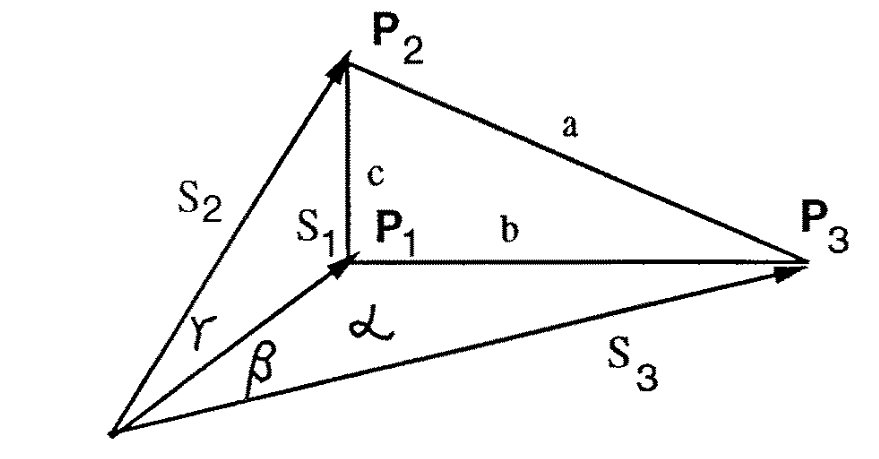
Figure 2: The P3P tetrahedron; \(P_{1}\), \(P_{2}\) and \(P_{3}\) are the unknown 3D points; \(a\), \(b\) and \(c\) are the known triangle sides, and the angles \(\alpha\), \(\beta\) and \(\gamma\) are also known. We need to solve for the lengths \(s_{1}\), \(s_{2}\), and \(s_{3}\). (credit: Haralick, Bert M., et al. “Review and analysis of solutions of the three point perspective pose estimation problem.” International journal of computer vision 13.3 (1994): 331-356.).
We know the lengths of the three bases (\(a\), \(b\) and \(c\)), where
\begin{align} a = || P_{2} - P_{3} || \\ b = || P_{1} - P_{3} || \\ c = || P_{1} - P_{2} || \end{align}Let the (calibrated) projections of \(P_{1}\), \(P_{2}\) and \(P_{3}\) be
\begin{align} q_{i} = \begin{bmatrix} u_{i} \\ v_{i} \\ 1 \end{bmatrix} \quad \text{where $i = 1, 2, 3$} \end{align}and the vectors pointing to the vertices of the bases from the optical center are therefore
\begin{align} P_{i} = s_{i} j_{i} = \frac{s_{i}}{\sqrt{u_{i}^{2} + v_{i}^{2} + 1}} \begin{bmatrix} u_{i} \\ v_{i} \\ 1 \end{bmatrix} \quad \text{where $i = 1, 2, 3$} \end{align}where \(s_{i}\) are the lengths of these vectors, and \(j_{i}\) are unit vectors.
We also define the following three angles (for convenience):
\begin{align} \cos \alpha=j_{2} \cdot j_{3} \\ \cos \beta=j_{1} \cdot j_{3} \\ \cos \gamma=j_{1} \cdot j_{2} \end{align}With these information, we need to calculate the lengths of these vectors (and the coordinates of the vertices \(P_{1}\), \(P_{2}\) and \(P_{3}\) of the bases come for free).
It is also possible to find \(R^{C}\) and \(t^{C}\) directly using linear algebra and geometry. The last method introduced in this post does this, and is perhaps the more widely used solver for P3P out there.
Grunert’s P3P
Grunert appears to present the first solution to the P3P problem in his 1841 work, Das Pothenotische Problem in erweiterter Gestalt nebst Über seine Anwendungen in der Geodäsie.
Using law of cosines, we have
\begin{align} s_{1}^{2} + s_{2}^{2} - 2 s_{1} s_{2} \cos{\gamma} = c^{2} \\ s_{1}^{2} + s_{3}^{2} - 2 s_{1} s_{3} \cos{\beta} = b^{2} \label{eq:p3p-system} \tag{1} \\ s_{2}^{2} + s_{3}^{2} - 2 s_{2} s_{3} \cos{\alpha} = a^{2} \\ \end{align}And the problem becomes how to solve for \(s_{1}\), \(s_{2}\) and \(s_{3}\) given the three equations above. Grunert employed a simple strategy of variable substitution: replacing \(s_{2}\) and \(s_{3}\) with \(s_{2} = u s_{1}\) and \(s_{3} = u s_{2}\). Using this substitution, the three equations above become:
\begin{align} s_{1}^{2} =\frac{c^{2}}{1+u^{2}-2 u \cos \gamma} \\ s_{1}^{2} =\frac{b^{2}}{1+v^{2}-2 v \cos \beta} \\ s_{1}^{2} =\frac{a^{2}}{u^{2}+v^{2}-2 u v \cos \alpha} \end{align}We then combine the equations containing \(\gamma\) and \(\beta\), and \(\beta\) and \(\alpha\) to get:
\begin{align} u^{2}-\frac{c^{2}}{b^{2}} v^{2}+2 v \frac{c^{2}}{b^{2}} \cos \beta -2 u \cos \gamma+\frac{b^{2}-c^{2}}{b^{2}}=0 \label{eq:beta-gamma} \tag{2} \end{align}and
\begin{align} u^{2}+\frac{b^{2}-a^{2}}{b^{2}} v^{2}-2 u v \cos \alpha +\frac{2 a^{2}}{b^{2}} v \cos \beta-\frac{a^{2}}{b^{2}}=0 \label{eq:alpha-beta} \tag{3} \end{align}From the Eq. \ref{eq:alpha-beta}, we can get an expression form \(u^{2}\):
\begin{align} u^{2}=-\frac{b^{2}-a^{2}}{b^{2}} v^{2}+2 u v \cos \alpha-\frac{2 a^{2}}{b^{2}} v \cos \beta+\frac{a^{2}}{b^{2}} \label{eq:grunert-u} \tag{4} \end{align}And substituting it back to Eq. \ref{eq:beta-gamma}, we have an expression for \(u\) in terms of \(v\):
\begin{align} u=\frac{\left(-1+\frac{a^{2}-c^{2}}{b^{2}}\right) v^{2}-2\left(\frac{a^{2}-c^{2}}{b^{2}}\right) \cos \beta v+1+\frac{a^{2}-c^{2}}{b^{2}}}{2(\cos \gamma-v \cos \alpha)} \end{align}This expression for \(u\) can then be substitute back to Eq. \ref{eq:alpha-beta} to get a polynomial in \(v\):
\begin{align} A_{4} v^{4} + A_{3} v^{3} + A_{2} v^{2} + A_{1} v + A_{0} = 0 \label{eq:grunert-poly} \tag{5} \end{align}where
\begin{align} A_{4}=&\left(\frac{a^{2}-c^{2}}{b^{2}}-1\right)^{2}-\frac{4 c^{2}}{b^{2}} \cos ^{2} \alpha \\ A_{3}=&4\left[\frac{a^{2}-c^{2}}{b^{2}}\left(1-\frac{a^{2}-c^{2}}{b^{2}}\right) \cos \beta -\left(1-\frac{a^{2}+c^{2}}{b^{2}}\right) \cos \alpha \cos \gamma +2 \frac{c^{2}}{b^{2}} \cos ^{2} \alpha \cos \beta\right] \\ A_{2}=&2\left[\left(\frac{a^{2}-c^{2}}{b^{2}}\right)^{2}-1+2\left(\frac{a^{2}-c^{2}}{b^{2}}\right)^{2} \cos ^{2} \beta+2\left(\frac{b^{2}-c^{2}}{b^{2}}\right) \cos ^{2} \alpha -4\left(\frac{a^{2}+c^{2}}{b^{2}}\right) \cos \alpha \cos \beta \cos \gamma + 2\left(\frac{b^{2}-a^{2}}{b^{2}}\right) \cos ^{2} \gamma\right] \\ A_{1}=&4\left[-\left(\frac{a^{2}-c^{2}}{b^{2}}\right)\left(1+\frac{a^{2}-c^{2}}{b^{2}}\right) \cos \beta +\frac{2 a^{2}}{b^{2}} \cos ^{2} \gamma \cos \beta -\left(1-\left(\frac{a^{2}+c^{2}}{b^{2}}\right)\right) \cos \alpha \cos \gamma\right] \\ A_{0}=& \left(1+\frac{a^{2}-c^{2}}{b^{2}}\right)^{2}-\frac{4 a^{2}}{b^{2}} \cos ^{2} \gamma \end{align}Eq. \ref{eq:grunert-poly} can have as many as four real solutions for \(v\). With each value of \(v\), we can easily recover the value of \(u\), which will then give us the values for \(s_{1}\), \(s_{2}\) and \(s_{3}\).
Note that there exists an algebraic singularity in this solution: when the denominator in Eq. \ref{eq:grunert-u} equals to zero. This will happen if \(\alpha = \beta = \gamma = 60 \deg\), and \(s_{1} = s_{2} = s_{3}\).
Fischler and Bolles’ P3P
Fischler and Bolles also presented a P3P solution in their seminal paper Random Sample Consensus: Random sample consensus: a paradigm for model fitting with applications to image analysis and automated cartography. Essentially, their derivation is similar to Grunert’s, except that they used a different set of algebraic manipulations to arrive at the final fourth order polynomial. In addition, their solution does not have an algebraic singularity.
Starting from the same P3P tetrahedron,
\begin{align} s_{1}^{2} =\frac{c^{2}}{1+u^{2}-2 u \cos \gamma} \\ s_{1}^{2} =\frac{b^{2}}{1+v^{2}-2 v \cos \beta} \\ s_{1}^{2} =\frac{a^{2}}{u^{2}+v^{2}-2 u v \cos \alpha} \end{align}they combined the second and third equations to get
\begin{align} v^{2} \left(1-\frac{a^{2}}{b^{2}}\right) +2 v \left(\frac{a^{2}}{b^{2}} \cos \beta-u\cos \alpha \right) +u^{2}-\frac{a^{2}}{b^{2}}=0 \label{eq:fischler-v2-1} \tag{6} \end{align}and they combined the first and third equations to get
\begin{align} v^{2}+2v(-\cos \alpha u) + u^{2}\left(1-\frac{a^{2}}{c^{2}}\right) + 2 u\frac{ a^{2}}{c^{2}} \cos \gamma -\frac{a^{2}}{c^{2}}=0 \label{eq:fischler-v2-2} \tag{7} \end{align}With Eq \ref{eq:fischler-v2-1} and \ref{eq:fischler-v2-2}, they observed that they can eliminate \(v\) by performing a few multiplications and substractions. Multiply Eq. \ref{eq:fischler-v2-1} by \(\left(1-\frac{a^{2}}{c^{2}}\right) u^{2}+\frac{2 a^{2}}{c^{2}} \cos \gamma u-\frac{a^{2}}{c^{2}}\), Eq. \ref{eq:fischler-v2-2} by \(u^{2}-\frac{a^{2}}{b^{2}}\), and subtract, we have
\begin{align} \left[\left(a^{2}-b^{2}-c^{2}\right) u^{2}+2\left(b^{2}-a^{2}\right) \cos \gamma u + \left(a^{2}-b^{2}+c^{2}\right)\right] v \\ + 2 b^{2} \cos \alpha u^{3} + \left(2\left(c^{2}-a^{2}\right) \cos \beta -4 b^{2} \cos \alpha \cos \gamma\right) u^{2} \\ + \left[4 a^{2} \cos \beta \cos \gamma + 2\left(b^{2}-c^{2}\right) \cos \alpha\right] u -2 a^{2} \cos \beta=0 \label{eq:fischler-v2-3} \tag{8} \end{align}Multiply Eq. \ref{eq:fischler-v2-2} by \(1 - \frac{a^{2}}{b^{2}}\), and subtract from Eq. \ref{eq:fischler-v2-1}, we have
\begin{align} 2 c^{2}(\cos \alpha u-\cos \beta) v+\left(a^{2}-b^{2}-c^{2}\right) u^{2} + 2\left(b^{2}-a^{2}\right) \cos \gamma u+a^{2}-b^{2}+c^{2}=0 \label{eq:fischler-v2-4} \tag{9} \end{align}Then, we multiply Eq. \ref{eq:fischler-v2-3} by \(2c^{2} (\cos{\alpha} u - \cos{\beta})\), and Eq. \ref{eq:fischler-v2-4} by \(\left[\left(a^{2}-b^{2}-c^{2}\right) u^{2}+2\left(b^{2}-a^{2}\right) \cos \gamma u+\left(a^{2}-b^{2}+c^{2}\right)\right]\), and subtract them to get
\begin{align} B_{4} u^{4}+B_{3} u^{3}+B_{2} u^{2}+B_{1} u+D_{0}=0 \label{eq:fischler-poly} \tag{10} \end{align}where
\begin{align} B_{4}=& 4 b^{2} c^{2} \cos ^{2} \alpha-\left(a^{2}-b^{2}-c^{2}\right)^{2} \\ B_{3}=&-4 c^{2}\left(a^{2}+b^{2}-c^{2}\right) \cos \alpha \cos \beta \\ &-8 b^{2} c^{2} \cos ^{2} \alpha \cos \gamma \\ &+4\left(a^{2}-b^{2}-c^{2}\right)\left(a^{2}-b^{2}\right) \cos \gamma \\ B_{2}=& 4 c^{2}\left(a^{2}-c^{2}\right) \cos ^{2} \beta \\ &+8 c^{2}\left(a^{2}+b^{2}\right) \cos \alpha \cos \beta \cos \gamma \\ &+4 c^{2}\left(b^{2}-c^{2}\right) \cos ^{2} \alpha \\ &-2\left(a^{2}-b^{2}-c^{2}\right)\left(a^{2}-b^{2}+c^{2}\right) \\ &-4\left(a^{2}-b^{2}\right)^{2} \cos ^{2} \gamma \\ B_{1}=&-8 a^{2} c^{2} \cos ^{2} \beta \cos \gamma \\ &-4 c^{2}\left(b^{2}-c^{2}\right) \cos \alpha \cos \beta \\ &-4 a^{2} c^{2} \cos \alpha \cos \beta \\ &+4\left(a^{2}-b^{2}\right)\left(a^{2}-b^{2}+c^{2}\right) \cos \gamma \\ B_{0}=& 4 a^{2} c^{2} \cos ^{2} \beta-\left(a^{2}-b^{2}+c^{2}\right)^{2} \end{align}As mentioned at the beginning, this solution to P3P does not have an algebraic singularity.
Gao’s P3P
The above two approaches are similar in the way of problem formulations: they both start with the law of cosines, and try to solve a system of polynomial solutions. A natural (perhaps more theoretical) extension is therefore how to systematically analyze what are all the possible solutions given the law of cosines equations. The paper Complete Solution Classification for the Perspective-Three-Point Problem by Xiao-Shan Gao et. al. does exactly this.
They start from the same system of equations (Eq. \ref{eq:p3p-system}), and add the following “reality conditions”, which correspond to geometrically nondegenerate solutions:
\begin{array}{l} s_{1}>0, s_{2}>0, s_{3}>0, a>0, b>0, c>0, a+b>c, a+c>b, b+c>a \\ 0<\alpha, \beta, \gamma<\pi, 0<\alpha+\beta+\gamma<2 \pi \\ \alpha+\beta>\gamma, \alpha+\gamma>\beta, \gamma+\beta>\alpha \\ I_{0}=(2 \cos \alpha)^{2}+ (2 \cos \beta)^{2}+ (2 \cos \gamma)^{2}- 8 \cos \alpha \cos \beta \cos \gamma-1 \neq 0 \end{array}They then proceed to simplify Eq. \ref{eq:p3p-system} by introducing \(x,y,z,r,p,q\), where \(x = s_{1} / s_{3}\), \(y = s_{2} / s_{3}\), \(v = ( c / s_{3})^{2}\), \(r = 2 \cos \gamma\), \(q = 2 \cos \beta\), \(p = 2 \cos \alpha\), \(a' = (a/s_{3})^{2} / v\), \(b' = (b / s_{3})^{2} / v\):
\begin{array}{r} y^{2}+1-y p-a' v=0 \\ x^{2}+1-x q-b' v=0 \\ x^{2}+y^{2}-x y r-v=0 \end{array}Then they eliminate \(v\) by substitution, reaching
\begin{array}{l} (1-a) y^{2}-a x^{2}-p y + arxy+1=0 \\ (1-b) x^{2}-b y^{2}-q x + brxy+1=0 \end{array}which are two quadratic equations, and therefore the P3P problem can only have either an infinite number of solutions or at most four physical solutions. For convenience, I will refer to this two equations as \(ES\) for the rest of this section.
To solve this two quadratic equations, they employ a method called Wu-Ritt’s zero decomposition. Essentially, it is a method for solving system of quadratic equations by first decomposing it into a series of equations in triangular forms:
\begin{equation} f_{1}\left(u, x_{1}\right)=0, f_{2}\left(u, x_{1}, x_{2}\right)=0, \ldots, f_{p}\left(u, x_{1}, \ldots, x_{p}\right)=0 \end{equation}where \(u\) are a set of parameters and \(x_{i}\) are the variables we are trying to solve. And the zero set of the original polynomial system is the union of zero sets of these triangular forms.
Using Wu-Ritt’s zero decomposition method, Gao and his colleagues decompose \(Zero(ES/I_{0})\) (which are the zero set of \(ES\) such that \(I_{0} \neq 0\)) into 10 disjoint components:
\begin{equation} \operatorname{Zero}\left(E S / I_{0}\right)=\bigcup_{i=1}^{10} \mathbf{C}_{i} \end{equation}where \(\mathbf{C}_{i}=\operatorname{Zero}\left(T S_{i} / T_{i}\right), i=1, \cdots, 9\) and \(C_{10}=\operatorname{Zero}\left(T S_{10} / T_{10}\right) \cup \operatorname{Zero}\left(T S_{11} / T_{11}\right)\). \(TS_{i}\) are polynomials in triangular form and \(T_{i}\) are polynomials.
If you want to see the exact expressions of these 10 components, you need to refer to their original paper. However, the key insight is that because the 10 components are disjoint, the solution therefore has to fall within 1 component only. In addition, within each component the parameters \(a'\), \(b'\), \(p\), \(q\) and \(r\) have to satisfy some algebraic conditions, which may correspond to the geometrically degenerate cases of P3P. Take \(TS_{4}\) as an example:
\begin{array}{l} \left(p^{2} b+q^{2} b-p^{2}\right) x^{2}+\left(-4 b q+p^{2} q\right) x+4 b-p^{2} \\ p y+q x-2 \\ a'+b'-1 \\ r \end{array}The equation \(a'+b'-1=0\) correspond to the case where \(\angle P_{1} P_{3} P_{2} = 90^{\circ}\). Thus to get the final solution, you just need to check all the 10 components and see which one is satisfied. In practice, the two implementations available for this method only return the solution to the main branch (see OpenCV’s implementation and OpenGV’s implementation).
Kneip P3P
Laurent Kneip in his 2011 paper A Novel Parametrization of the Perspective-Three-Point Problem for a Direct Computation of Absolute Camera Position and Orientation proposes yet another P3P solution. The unique part of his method comparing to the aforementioned 3 methods is that it directly solves for the rotation and translation through a clever parametrization of the problem.
Let’s go over this method step by step. First, we need to define two new reference frames: one oriented on the bearing vectors of the three known projections of the three 3D points (\(\tau\)), and one oriented on the three 3D points directly (\(\eta\)).
In the following section, to avoid confusion with the paper, we define \(\vec{f}_{1} = \vec{s}_{1}\), \(\vec{f}_{2} = \vec{s}_{2}\) and \(\vec{f}_{3} = \vec{s}_{3}\). Define \(\tau\)’s axes as
\begin{align} \vec{t}_{x}&=\vec{f}_{1} \\ \vec{t}_{z}&=\frac{\vec{f}_{1} \times \vec{s}_{2}}{\left\|\vec{f}_{1} \times \vec{f}_{2}\right\|} \\ \vec{t}_{y}&=\vec{t}_{z} \times \vec{t}_{x} . \end{align}and \(\tau\)’s origin is the camera center in the world frame. If we define \(T=\left[\vec{t}_{x}, \vec{t}_{y}, \vec{t}_{z}\right]^{T}\), then the bearing vectors of the input 2D points (in the camera’s frame) can be transformed into \(\tau\) by:
\begin{align} \vec{f}_{i}^{\tau}=T \cdot \vec{f}_{i} \end{align}Define \(\eta\)’s axes as
\begin{align} \vec{n}_{x}&=\frac{\overrightarrow{P_{1} P}_{2}}{\left\|\overrightarrow{P_{1} P}_{2}\right\|} \\ \vec{n}_{z}&=\frac{\vec{n}_{x} \times \overrightarrow{P_{1} P}_{3}}{\left\|\vec{n}_{x} \times \overrightarrow{P_{1} P}_{3}\right\|} \\ \vec{n}_{y}&=\vec{n}_{z} \times \vec{n}_{x} \end{align}and with its origin be \(P_{1}\). Note that these axes and the origin are in the fixed world frame. If we define \(N =\left[\vec{n}_{x}, \vec{n}_{y}, \vec{n}_{z}\right]^{T}\), then it follows that we can transform the world points \(P_{i}\) into \(\eta\) as:
\begin{align} P^{\eta}_{i} = N ( P_{i} - P_{1} ) \end{align}Note that the condition \(\overrightarrow{P_{1} P}_{2} \times \overrightarrow{P_{1} P}_{3}\) has to be satisfied (\(P_{1}\), \(P_{2}\) and \(P_{3}\) not colinear).
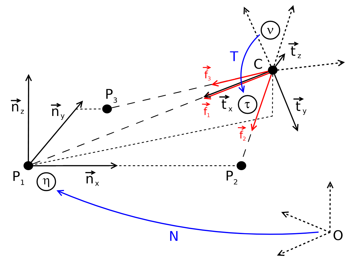
Figure 3: Illustration of \(\eta\) and \(\tau\). Note that \(f_{1}\), \(f_{2}\) and \(f_{3}\) are equivalent with our previously defined \(s_{1}\), \(s_{2}\) and \(s_{3}\). (credit: Kneip, Laurent, Davide Scaramuzza, and Roland Siegwart. “A novel parametrization of the perspective-three-point problem for a direct computation of absolute camera position and orientation.” CVPR 2011. IEEE, 2011.)
After we have the two intermediate frames, we only need to find the transformation between them to recover the relative transformation between the fixed world frame and the camera frame. The rest of the method therefore focuses on finding the transformation between \(\eta\) and \(\tau\).
To identify the transformation, we need to find the coordinates of \(C\) (origin of the \(\tau\) frame) in the \(\eta\) frame, as well as a rotation matrix that align the two sets of axes. First, let’s find the coordinates of \(C\) in \(\eta\). Note that if we construct a plane \(\Pi\) containing the points \(P_{1}\), \(P_{2}\) and \(C\) (Fig. 4), we can describe \(C\)’s coordinate on that plane based on the distance between \(P_{1}\) and \(P_{2}\), the angle between \(f_{1}\) and \(f_{2}\), which are both known and fixed, and lastly the angle between \(P_{1} C\) and \(P_{1} P_{2}\), which is unknown. And together with the angle formed between the plane \(\Pi\) and the plane spanned by \(\vec{n}_{x}\) and \(\vec{n}_{y}\), we can write down an expression for \(C\) in \(\eta\) frame.
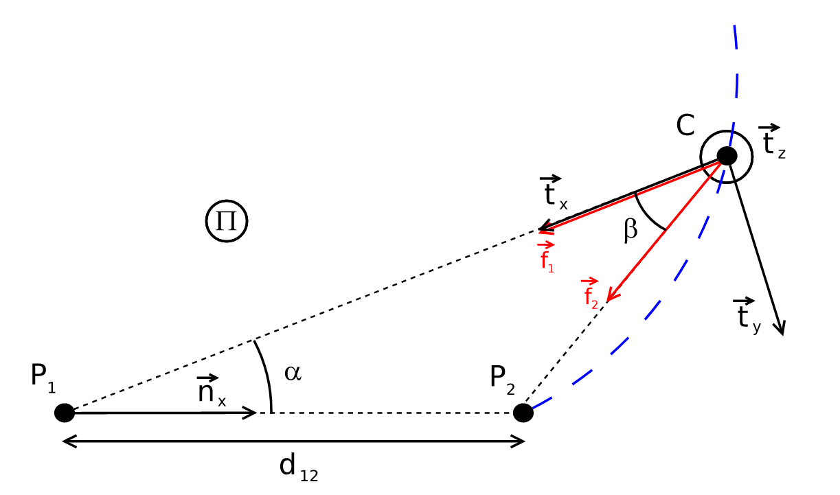
Figure 4: Plane \(\Pi\) containing the points \(P_{1}\), \(P_{2}\) and \(C\). (credit: Kneip, Laurent, Davide Scaramuzza, and Roland Siegwart. “A novel parametrization of the perspective-three-point problem for a direct computation of absolute camera position and orientation.” CVPR 2011. IEEE, 2011.)
So it follows that we can define a \(b\) such that
\begin{align} b=\cot \beta=\pm \sqrt{\frac{1}{1-\cos ^{2} \beta}-1}=\pm \sqrt{\frac{1}{1-\left(\vec{f}_{1} \cdot \vec{f}_{2}\right)^{2}}-1} \end{align}and \(\cos{\beta} = \vec{f}_{1} \cdot \vec{f}_{2}\). Then, define \(\alpha=\angle P_{2} P_{1} C\), and we have
\begin{align} \frac{\left\|\overrightarrow{C P}_{1}\right\|}{d_{12}}=\frac{\sin (\pi-\alpha-\beta)}{\sin \beta} \end{align}and the position of \(C\) in \(\Pi\)’s frame (with \(P_{1}\) as the origin, \(\vec{n}_{x}\) as the $x$-axis, $z$-axis perpendicular on the plane) is therefore
\begin{align} C^{\Pi}(\alpha) &=\left(\begin{array}{c} \cos \alpha \cdot\left\|\overrightarrow{C P}_{1}\right\| \\ \sin \alpha \cdot\left\|\overrightarrow{C P}_{1}\right\| \\ 0 \end{array}\right) \\ &=\left(\begin{array}{c} d_{12} \cos \alpha \sin (\alpha+\beta) \sin ^{-1} \beta \\ d_{12} \sin \alpha \sin (\alpha+\beta) \sin ^{-1} \beta \\ 0 \end{array}\right) \\ &=\left(\begin{array}{c} d_{12} \cos \alpha(\sin \alpha \cot \beta+\cos \alpha) \\ d_{12} \sin \alpha(\sin \alpha \cot \beta+\cos \alpha) \\ 0 \end{array}\right) \end{align}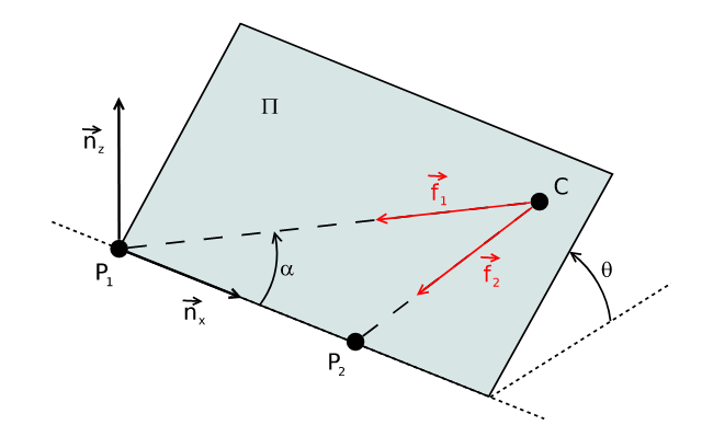
Figure 5: Rotation of plane \(\Pi\) around \(\vec{n}_{x}\) by \(\theta\). (credit: Kneip, Laurent, Davide Scaramuzza, and Roland Siegwart. “A novel parametrization of the perspective-three-point problem for a direct computation of absolute camera position and orientation.” CVPR 2011. IEEE, 2011.)
The rotation of plane \(\Pi\) around \(\vec{n}_{x}\) (Fig. 5) can be expressed as the following rotation matrix (just an elementary rotation matrix around the $x$-axis):
\begin{align} C^{\eta}(\alpha, \theta) &=R_{\theta} \cdot C^{\Pi} \\ &=\left(\begin{array}{c} d_{12} \cos \alpha(\sin \alpha \cdot b+\cos \alpha) \\ d_{12} \sin \alpha \cos \theta(\sin \alpha \cdot b+\cos \alpha) \\ d_{12} \sin \alpha \sin \theta(\sin \alpha \cdot b+\cos \alpha) \end{array}\right) \end{align}Note how this matrix’s columns are the expressions of the new axes (\(\eta\) frame’s axes) in the old frame (plane \(\Pi\)’s frame). So we have the coordinate of \(C\) in \(\eta\) as:
\begin{align} C^{\eta}(\alpha, \theta) &=R_{\theta} \cdot C^{\Pi} \\ &=\left(\begin{array}{c} d_{12} \cos \alpha(\sin \alpha \cdot b+\cos \alpha) \\ d_{12} \sin \alpha \cos \theta(\sin \alpha \cdot b+\cos \alpha) \\ d_{12} \sin \alpha \sin \theta(\sin \alpha \cdot b+\cos \alpha) \end{array}\right) \end{align}Now that we have \(C^{\eta}\), we only need the rotation matrix describing transformation from \(\eta\) to \(\tau\). It turns out that it’s easier for us to get the rotation from \(\tau\) to \(\eta\) first, then take the transpose. For that, we need to find out the expressions for \(\vec{t}_{x}\), \(\vec{t}_{y}\) and \(\vec{t}_{z}\) in \(\tau\). It follows that we have
\begin{align} R_{\eta}^{\tau} &= \left[ R_{\theta} \cdot\left(\vec{t}_{x}^{\Pi} | \vec{t}_{y}^{\Pi} | \vec{t}_{z}^{\Pi}\right) \right] = \left(\begin{array}{ccc} -\cos \alpha & -\sin \alpha \cos \theta & \sin \alpha \\ -\sin \alpha \sin \theta & -\cos \alpha \cos \theta & -\sin \theta \\ 0 & -\cos \alpha \sin \theta & \cos \theta \end{array}\right) \end{align}And therefore we have
\begin{align} Q(\alpha, \theta) = R_{\tau}^{\eta} = \left(\begin{array}{ccc} -\cos \alpha & -\sin \alpha \cos \theta & -\sin \alpha \sin \theta \\ \sin \alpha & -\cos \alpha \cos \theta & -\cos \alpha \sin \theta \\ 0 & -\sin \theta & \cos \theta \end{array}\right) \end{align}With \(Q(\alpha, \theta)\) defined, we now need to write down the systems of equations to solve for \(\alpha\) and \(\theta\). To do that, we simply write out the equations for transforming \(P^{\eta}_{3}\) into \(P^{\tau}_{3}\). Let \(P^{\eta}_{3} = (p_{1}, p_{2}, 0)^{T}\) (which is known), it follows that
\begin{align} \begin{array}{c} P_{3}^{\tau}=Q(\alpha, \theta) \cdot\left(P_{3}^{\eta}-C^{\eta}(\alpha, \theta)\right) \\ =\left(\begin{array}{c} -\cos \alpha \cdot p_{1}-\sin \alpha \cos \theta \cdot p_{2}+d_{12}(\sin \alpha \cdot b+\cos \alpha) \\ \sin \alpha \cdot p_{1}-\cos \alpha \cos \theta \cdot p_{2} \\ -\sin \theta \cdot p_{2} \end{array}\right) \end{array} \end{align}In addition, notice that the direction of \(P^{\tau}_{3}\) is the same as that of \(\vec{f}^{\tau}_{3}\) (also known). Define
\begin{align} \phi_{1}=\frac{f_{3, x}^{\tau}}{f_{3, z}^{\tau}}, \qquad \phi_{2}=\frac{f_{3, y}^{\tau}}{f_{3, z}^{\tau}} \end{align}It follows that
\begin{align} &\left\{\begin{array}{l} \phi_{1}=\frac{P_{3, x}^{\tau}}{P_{3}^{\tau} z} \\ \phi_{2}=\frac{P_{3, y}^{\tau}}{P_{3, z}^{\tau}} \end{array}\right. \\ \Rightarrow & \left\{\begin{array}{l} \phi_{1}=\frac{-\cos \alpha \cdot p_{1}-\sin \alpha \cos \theta \cdot p_{2}+d_{12}(\sin \alpha \cdot b+\cos \alpha)}{-\sin \theta \cdot p_{2}} \\ \phi_{2}=\frac{\sin \alpha \cdot p_{1}-\cos \alpha \cos \theta \cdot p_{2}}{-\sin \theta \cdot p_{2}} \end{array}\right. \\ \Rightarrow & \left\{\begin{array}{l} \frac{\sin \theta}{\sin \alpha} p_{2}=\frac{-\cot \alpha \cdot p_{1}-\cos \theta \cdot p_{2}+d_{12}(b+\cot \alpha)}{-\phi_{1}} \\ \frac{\sin \theta}{\sin \alpha} p_{2}=\frac{p_{1}-\cot \alpha \cos \theta \cdot p_{2}}{-\phi_{2}} \end{array}\right. \\ \Rightarrow & \cot \alpha=\frac{\frac{\phi_{1}}{\phi_{2}} p_{1}+\cos \theta \cdot p_{2}-d_{12} \cdot b}{\frac{\phi_{1}}{\phi_{2}} \cos \theta \cdot p_{2}-p_{1}+d_{12}} \label{eq:cot-alpha} \tag{11} \end{align}In addition, from definition of \(\phi_{2}\), we also have
\begin{align} \sin ^{2} \theta \cdot f_{2}^{2} p_{2}^{2}=\sin ^{2} \alpha\left(p_{1}-\cot \alpha \cos \theta \cdot p_{2}\right)^{2} \\ \left(1-\cos ^{2} \theta\right)\left(1+\cot ^{2} \alpha\right) f_{2}^{2} p_{2}^{2} =p_{1}^{2}-2 \cot \alpha \cos \theta \cdot p_{1} p_{2}+\cot ^{2} \alpha \cos ^{2} \theta \cdot p_{2}^{2} \label{eq:kneip-polynomial-before} \tag{12} \end{align}Substitute Eq. \ref{eq:cot-alpha} into Eq. \ref{eq:kneip-polynomial-before}, we have
\begin{align} a_{4} \cdot \cos ^{4} \theta+a_{3} \cdot \cos ^{3} \theta+a_{2} \cdot \cos ^{2} \theta+a_{1} \cdot \cos \theta+a_{0}=0 \label{eq:kneip-polynomial-after} \tag{13} \end{align}where
\begin{align} a_{4}=&-\phi_{2}^{2} p_{2}^{4}-\phi_{1}^{2} p_{2}^{4}-p_{2}^{4} \\ a_{3}=& 2 p_{2}^{3} d_{12} b+2 \phi_{2}^{2} p_{2}^{3} d_{12} b-2 \phi_{1} \phi_{2} p_{2}^{3} d_{12} \\ a_{2}=&-\phi_{2}^{2} p_{1}^{2} p_{2}^{2}-\phi_{2}^{2} p_{2}^{2} d_{12}^{2} b^{2}-\phi_{2}^{2} p_{2}^{2} d_{12}^{2}+\phi_{2}^{2} p_{2}^{4} \\ &+\phi_{1}^{2} p_{2}^{4}+2 p_{1} p_{2}^{2} d_{12}+2 \phi_{1} \phi_{2} p_{1} p_{2}^{2} d_{12} b \\ &-\phi_{1}^{2} p_{1}^{2} p_{2}^{2}+2 \phi_{2}^{2} p_{1} p_{2}^{2} d_{12}-p_{2}^{2} d_{12}^{2} b^{2}-2 p_{1}^{2} p_{2}^{2} \\ a_{1}=& 2 p_{1}^{2} p_{2} d_{12} b+2 \phi_{1} \phi_{2} p_{2}^{3} d_{12} \\ &-2 \phi_{2}^{2} p_{2}^{3} d_{12} b-2 p_{1} p_{2} d_{12}^{2} b \\ a_{0}=&-2 \phi_{1} \phi_{2} p_{1} p_{2}^{2} d_{12} b+\phi_{2}^{2} p_{2}^{2} d_{12}^{2}+2 p_{1}^{3} d_{12} \\ &-p_{1}^{2} d_{12}^{2}+\phi_{2}^{2} p_{1}^{2} p_{2}^{2}-p_{1}^{4}-2 \phi_{2}^{2} p_{1} p_{2}^{2} d_{12} \\ &+\phi_{1}^{2} p_{1}^{2} p_{2}^{2}+\phi_{2}^{2} p_{2}^{2} d_{12}^{2} b^{2} \end{align}We can solve Eq. \ref{eq:kneip-polynomial-after} in closed form for \(\cos{\theta}\), and using Eq. \ref{eq:cot-alpha} to recover \(\cot{\alpha}\). With \(\alpha\), and \(\theta\), we can then calculate \(C\) and \(Q\) to recover the camera center and orientation with respect to the world frame:
\begin{align} C=P_{1}+N^{T} \cdot C^{\eta} \\ R=N^{T} \cdot Q^{T} \cdot T \end{align}Implementation
References
See the following papers:
- B. M. Haralick, C.-N. Lee, K. Ottenberg, and M. Nölle, “Review and analysis of solutions of the three point perspective pose estimation problem,” Int J Comput Vision, vol. 13, no. 3, pp. 331–356, Dec. 1994, doi: 10.1007/BF02028352.
- L. Kneip, D. Scaramuzza, and R. Siegwart, “A novel parametrization of the perspective-three-point problem for a direct computation of absolute camera position and orientation,” in CVPR 2011, Jun. 2011, pp. 2969–2976. doi: 10.1109/CVPR.2011.5995464.
- X.-S. Gao, X.-R. Hou, J. Tang, and H.-F. Cheng, “Complete solution classification for the perspective-three-point problem,” IEEE Transactions on Pattern Analysis and Machine Intelligence, vol. 25, no. 8, pp. 930–943, Aug. 2003, doi: 10.1109/TPAMI.2003.1217599.
For Kneip’s P3P algorithm, I also referenced his excellent OpenGV library.