Panorama: How?
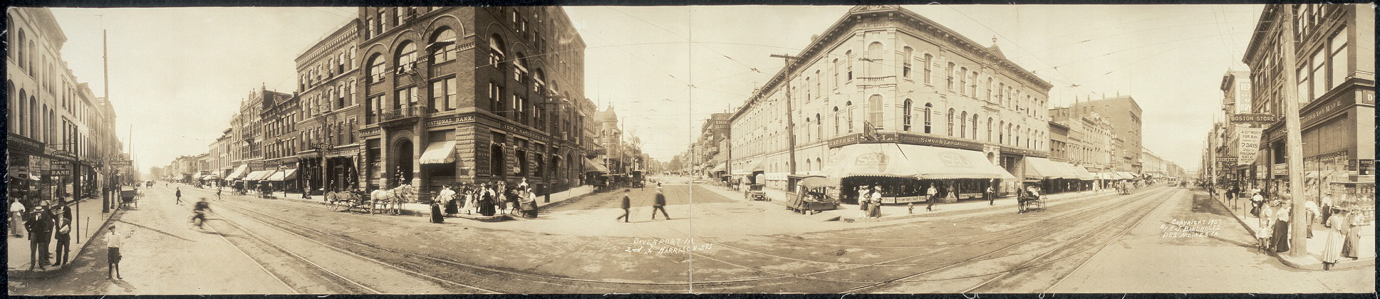
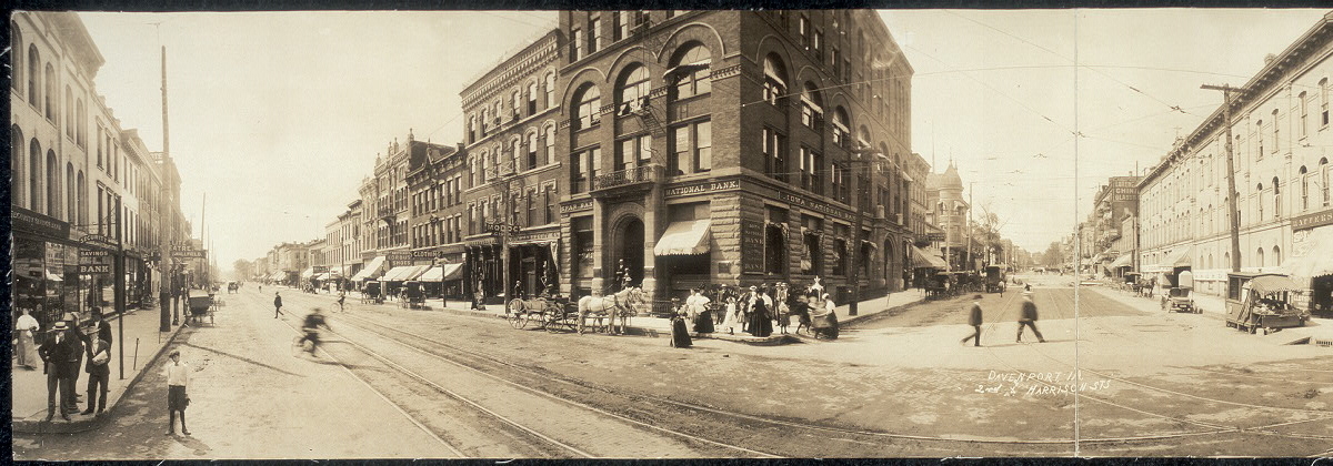
Figure 1: Davenport, IA, 2nd & Harrison Sts.; c1907 F.J. Bandholtz gelatin silver print; 10 x 47 in. PAN US GEOG - Iowa, no. 48 (E size) P&P. Courtesy of Library of Congress.
Have you ever wondered how a photo like Fig. 1 is shot? In this blog post, I will walk you through the early mechanical panoramic cameras, show you the math behind compositing panoramic shots, and present a demo of making your own panoramic shots with a few lines of code.
The Mechanical
Burlington, Wisconsin is a town located right at the confluence of the White and Fox rivers. Established as a village in 1886 1, Burlington is the home of one of the first commercially available panoramic cameras, the Al-Vista camera.
The patent for the Al-Vista camera was filed by Peter N. Angsten of Burlington and Charles H. Gesbeck of Chicago, on May 31st 1898 2.
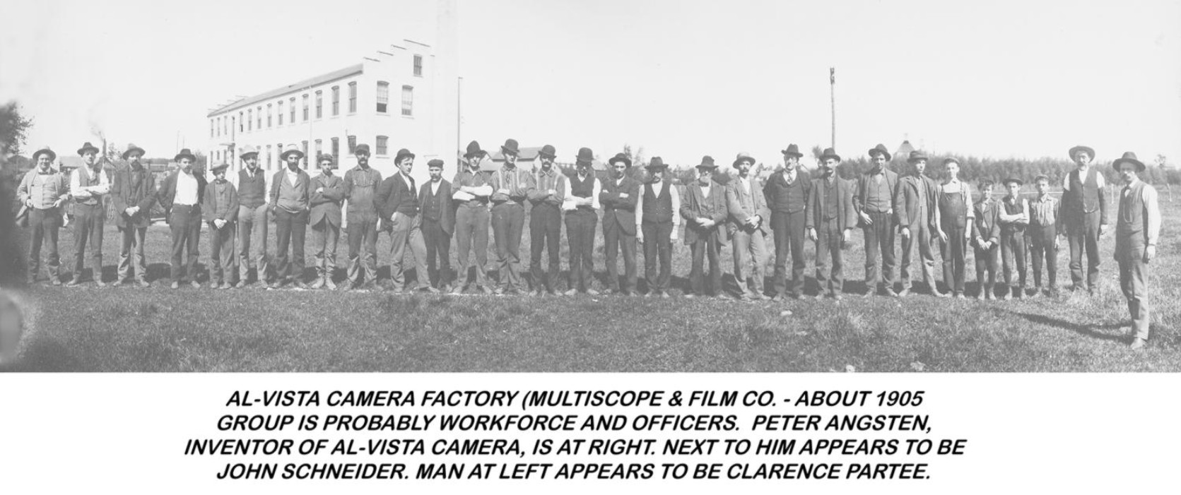
Figure 2: Peter Angsten and some other employees at the Multiscope And Film Co., courtesy of Burlington Historical Society (source).
Peter was employed by the Multiscope And Film Co., which was a company manufacturing cameras and camera outfits located on the interfaction of Calumet St. and Jefferson, on the White river bank.
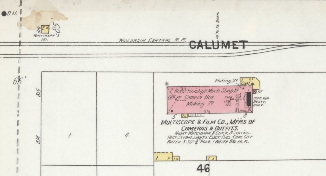
Figure 3: The Multiscope And Film Co. factory on a 1904 fire insurance map
The camera itself has an ingenious design. One of its advertisements said3:
Sweeps the Field. Takes everything in sight, rotating in such a way as to take a series of separate views, covering an area of one hundred and eighty degrees. The most wonderful of modern cameras.
It has a spring-loaded spindle that rotates the lens holder horizontally from left to right. The spindle can be adjusted for tension such that the exposure duration can be changed.
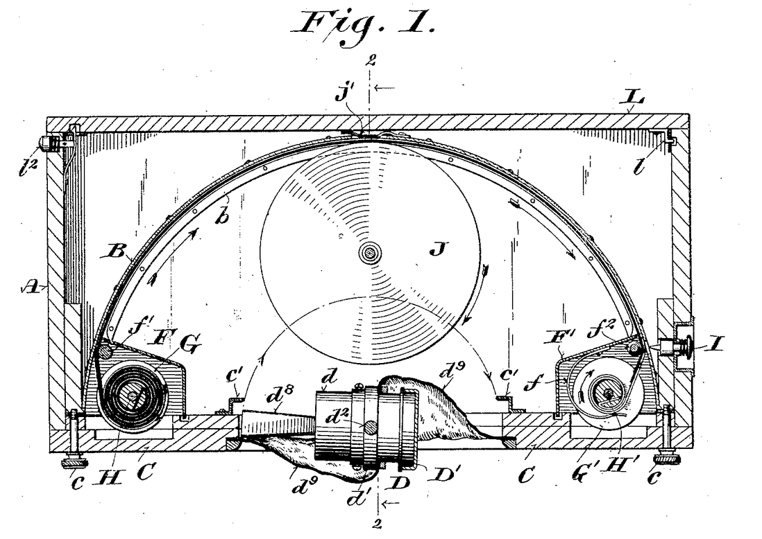
Figure 4: A schematic on the patent showing the spring-loaded spindle and the lens holder
Al-Vista was certainly not the only panoramic camera on the market during the early 1900s. In 1904, the Cirkut camera was patented.
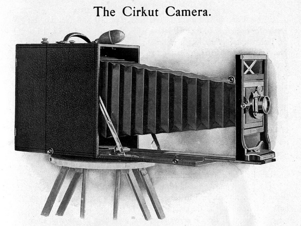
Figure 5: A schematic of the Cirkut camera, source.
Instead of being a hand-held camera like Al-Vista, the Cirkut camera stands on a tripod. According to a 1900s camera catlog4:
The Cirkut Panoramic Outfit is in itself a most complete affair, … In addition it contains the mechanism which, when the outfit is in operation, unwinds the film past a slot on a roller and in so doing exposes it and at the same time revolves the camera about on an axis, a special tripod and top being furnished.
The main idea behind these two models of panoramic camera is the same: by rotating the lens, the projected image of the scene can horizontally pans across the film. In doing so, such cameras are restricted to take only panning panoramas that are long rectangular strips of image. While restricted in motion, these cameras nevertheless produce stunning images on the hands of skilled photographers5.
Physically, I don’t see any restrictions on designing a film camera that can take arbitrary shapes of panorama. Perhaps instead of rotating the camera lens around the yaw axis, we can design a ball head similar to those of tripods that allow rotations in three degrees of freedom.
Alas, I am no expert in manufacturing (I have been eyeing for a 3D printer for ages. I still haven’t made up my minds on the model to buy.) Nevertheless, I do know a bit of math and principles of pinhole cameras. So let’s see whether we can figure something out in math and write code to make our own panoramas.
The Mathematics
The main idea behind virtually stitching images together to make panoramas is to find relative transformations. by figuring out the relative rotation between cameras of consecutive images.

Figure 6: A schematic showing a pinhole camera with its axes.
I am going to use the standard ideal perspective camera model for the following sections. I will talk a lot about three reference frames: the world frame \(W\), the camera frame \(C\), and the image frame. You can think of the world frame as the global coordinate frame the camera and the objects live in. The camera frame is a coordinate frame attached to the camera with the origin at the optical center. The image frame is simply a 2D coordinate frame attached to the top-left corner of the image plane.
The image formation process under an ideal perspective model follows Eq. \ref{eq:pinhole}:
\begin{align} z \tilde{x} = \mathbf{K} \begin{bmatrix} \mathbf{R}^{C}_{W} & \mathbf{t}^{C}_{W} \end{bmatrix} p^W \label{eq:pinhole} \tag{1} \end{align}where \(\mathbf{K}\) denotes the camera intrinsic matrix, \(\tilde{x}\) is the 2D image point, \(\tilde{p}^{W}\) is the 3D point in the world frame, and \((\mathbf{R}^{C}_{W}, \mathbf{t}^{C}_{W})\) is the 3D rotation and translation of the camera frame with respect to the world frame. \(z\) is a scalar value that equals to the \(z\) coordinate of \(\begin{bmatrix} \mathbf{R}^{C}_{W} & \mathbf{t}^{C}_{W} \end{bmatrix} p^{W}\), and it represents the depth of the point in the camera frame (usually unknown).
To clarify the notations a bit more:
- I use superscripts to denote the coordinates frames in which vectors live.
- For rotations and translations, the subscripts indicate the frames from which they transform, and the superscripts indicate the frames to which they transform. This way the subscripts of \(\mathbf{R}\) can sort of “cancel out” the superscripts of vectors.
- \({\large \tilde{\cdot}}\) means homogeneous coordinates.

Figure 7: A schematic showing two cameras viewing the same point \(p\)
With the preliminaries out of the way, I will now start discussing the case with two cameras. In our case, the two cameras are snapshots of the same camera at two different time instants. For our convenience, instead of using a separate world frame I use the camera frame of the left camera (camera 1) as the world frame. In other words, the \((\mathbf{R}, \mathbf{t})\) terms in Eq. \ref{eq:pinhole} are the 3-by-3 identity matrix and zero vector. Thus for camera 1, we have: \[ z_{1} \tilde{\mathbf{x}}_{1}=\mathbf{K}\left[\mathbf{I}_{3} \vert \mathbf{0}_{3}\right] \tilde{\mathbf{p}}^{\mathrm{c}_{1}}=\mathbf{K}_{1} \mathbf{p}^{\mathrm{c}_{1}} \] For camera 2, we have: \[ z_{2} \tilde{\mathbf{x}}_{2}=\mathbf{K}\left[\mathbf{R} \vert \mathbf{t}_{\mathrm{c}_{1}}^{\mathrm{c}_{2}}\right] \tilde{\mathbf{p}}^{\mathrm{c}_{1}} \] Define \(\mathbf{y}_{1} = \mathbf{K}^{-1} \tilde{\mathbf{x}}_{1}\) and \(\mathbf{y}_{2} = \mathbf{K}^{-1} \tilde{\mathbf{x}}_{2}\). Then we have
\begin{align} z_{1} \tilde{\mathbf{y}_{1}} = p^{c_{1}} \label{eq:cam1-calib-img-formation} \tag{2} \end{align}and
\begin{align} z_{2} \tilde{\mathbf{y}}_{2} = R p^{c_{1}} + \mathbf{t} \label{eq:cam2-calib-img-formation} \tag{3} \end{align}Substitute Eq. \ref{eq:cam1-calib-img-formation} into \ref{eq:cam2-calib-img-formation}, we have
\begin{align} z_{2} \tilde{\mathbf{y}}_{2} = R z_{1} \tilde{\mathbf{y}_{1}} + \mathbf{t} \label{eq:after-substitution} \tag{4} \end{align}Use the fact that a vector’s cross product with itself equals to zero, and the fact that cross product can be represented as a pre-multiplication of a skew-symmetric matrix (denoted by \([{\large \cdot}]_{\times}\)), we have \[ z_{2} [\mathbf{t}]_{\times} \tilde{\mathbf{y}}_{2} = z_{1} [\mathbf{t}]_{\times} \mathbf{R} \tilde{\mathbf{y}}_{1} \] Premultiply by \(\mathbf{y}_{2}^{T}\), and use the fact that \([\mathbf{t}]_{\times} \tilde{\mathbf{y}}_{2}\) is orthogonal to \(\tilde{\mathbf{y}}_{2}\), we have \[ \tilde{\mathbf{y}}_{2}^{T} [\mathbf{t}]_{\times} \mathbf{R} \tilde{\mathbf{y}}_{1} = 0 \] We have just derived out the famous epipolar constraint, and \(\mathbf{E} = [\mathbf{t}]_{\times} \mathbf{R}\) is the essential matrix. However, for rotational panoramas, we have \(\mathbf{t} = \mathbf{0}\), which will essentially render the above equation useless.
To adapt to the zero translation case, we just need to go back to Eq. \ref{eq:cam2-calib-img-formation}. Because we already know that \(\mathbf{t}\) is zero, Eq. \ref{eq:cam2-calib-img-formation} can be rewritten as:
\begin{align} \mathbf{R} \tilde{\mathbf{y}}_{1} = c \tilde{\mathbf{y}}_{2} \label{eq:parallel-lines-1} \tag{5} \end{align}where \(c\) is an arbitrary constant. This is essentially saying that \(\mathbf{R} \tilde{\mathbf{y}}_{1}\) is parallel to \(\tilde{\mathbf{y}}_{2}\).
Note that we can get something similar by going back to Eq. \ref{eq:after-substitution} as well. Because we already know that \(\mathbf{t}\) is zero, we no longer need to pre-multiply it by \([\mathbf{t}]_{\times}\). Instead, we pre-multiply the equation by \([\tilde{\mathbf{y}}_{2}]_{\times}\):
\begin{align} [\tilde{\mathbf{y}}_{2}]_{\times} \mathbf{R} \tilde{\mathbf{y}}_{1} = \mathbf{0} \label{eq:parallel-lines-2} \tag{6} \end{align}Eq. \ref{eq:parallel-lines-1} and \ref{eq:parallel-lines-2} are equivalent.
Now, if you are familiar with the concept of planar homography matrix, you will realize that Eq.~\ref{eq:parallel-lines-2} is suspiciously similar to the constraint for planar homography matrices: \[ [\tilde{\mathbf{y}}_{2}]_{\times} \mathbf{H} \tilde{\mathbf{y}}_{1} = \mathbf{0} \] And \[ \mathbf{H} \doteq \mathbf{R} + \frac{1}{d} \mathbf{t} \mathbf{N}^{T} \] where \(N\) is the normal vector of the plane in camera frame, and \(d\) is the distance from the plane to camera center. In fact, in the case for pure rotations, we can treat \(d\) to be effectively equal to infinity, thus making \(\mathbf{H} \approx \mathbf{R}\). As a result, we can use the machinery provided in OpenCV, which I will present in the next section.
The Code
Based on the previous discussions, we can come up with a script pretty easily:
import numpy as np
import cv2


def get_matches(img1, img2):
    # find SIFT features
    sift_finder = cv2.SIFT_create()
    kpts_1, des_1 = sift_finder.detectAndCompute(img1, None)
    kpts_2, des_2 = sift_finder.detectAndCompute(img2, None)

    # nearest neighbor matching
    matcher = cv2.DescriptorMatcher_create(cv2.DESCRIPTOR_MATCHER_FLANNBASED)
    raw_matches = matcher.knnMatch(des_1, des_2, 2)

    # use ratio test to pick good matches
    good_matches = []
    for m, n in raw_matches:
        if m.distance < 0.7 * n.distance:
            good_matches.append(m)

    return kpts_1, kpts_2, good_matches


def to_points(kpts_1, kpts_2, matches):
    # pick the matched points
    img1_pts = np.float32([kpts_1[m.queryIdx].pt for m in matches]).reshape(-1, 2)
    img2_pts = np.float32([kpts_2[m.trainIdx].pt for m in matches]).reshape(-1, 2)

    return img1_pts,img2_pts


def stitch(img1, img2, H):
    img_width = img1.shape[1]
    img_height = img1.shape[0]
    panorama_width = img_width * 2
    panorama_height = img_height * 2

    # put img2 to panorama
    panorama = np.zeros((panorama_height, panorama_width, 3))
    panorama[0:img2.shape[0], 0:img2.shape[1], :] = img2

    # mask out img2
    mask = np.ones((panorama_height, panorama_width, 1))
    mask[0:img2.shape[0], 0:img2.shape[1], :] = np.zeros((img2.shape[0], img2.shape[1], 1))

    # add warped img1
    img1_warped = cv2.warpPerspective(img1, H, (panorama_width, panorama_height))*mask
    panorama = panorama + img1_warped

    # crop
    rows, cols = np.where(panorama[:, :, 0] != 0)
    min_row, max_row = min(rows), max(rows) + 1
    min_col, max_col = min(cols), max(cols) + 1
    final_panorama = panorama[min_row:max_row, min_col:max_col, :]

    return final_panorama


if __name__ == "__main__":
    # images to use for panorama
    img1 = cv2.imread("davenport-right.jpg")
    img2 = cv2.imread("davenport-left.jpg")

    # find correspondences
    kpts_1, kpts_2, good_matches = get_matches(img1, img2)
    pts_1, pts_2 = to_points(kpts_1, kpts_2, good_matches)

    # find homography & warp image
    H, status = cv2.findHomography(pts_1, pts_2, cv2.RANSAC,5.0)

    panorama = stitch(img1, img2, H)
    cv2.imwrite("panorama.jpg", panorama)
It first uses SIFT feature descriptors to find matching points, and then estimate the homography matrix between them 6. Overall, OpenCV is doing the heavy lifting, so we can finish the script within a hundred lines.
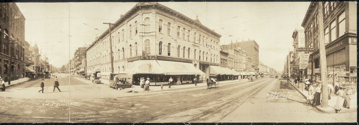
I split Fig. 1 into two (download them from here and here), and fed them into the script above. The resulting image is shown below:
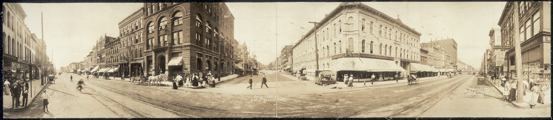
Figure 8: The output panorama from running the code above. It looks exactly like Fig. 1!
Now you have your own digital Al-Vista camera!
Footnotes:
See here for the actual patent https://patents.google.com/patent/US778394
For more old panoramic photos, visit http://www.panoramicphoto.com/.
See here for a tutorial on homography, specifically for the section of the pure rotational case: https://docs.opencv.org/master/d9/dab/tutorial_homography.html